WORKING PAPER · PART 2 · FROM COAL-EQUIVALENT PLANTS TO A COAL-EQUIVALENT FLEET
Geographic Diversification at Continental Scale
Contents30 sections
Summary
A geographically distributed fleet of solar-plus-storage plants can deliver firm, round-the-clock power at continental scale through the same mechanism that makes coal fleets reliable. Individual coal units are rated at only ~ 85% availability, yet because their forced outages are largely uncorrelated the fleet meets demand in over 99% of hours; solar-plus-storage shortfalls, driven by local weather that decorrelates across India’s 3,000 km span, obey the same portfolio logic. The northwest has India’s strongest solar resource; the northeast tends to have clearer skies when western India is under heavy monsoon rain; and the south’s rainy season (October–December) falls outside the June–September monsoon affecting the rest of India. These offsets ensure that no single weather system can suppress output across the entire fleet.
We simulate 120 DC-coupled plants (5.0 GW-AC solar + 17.78 GWh nameplate battery / 16 GWh usable each) distributed across 18 Indian states: 600 GW-AC of solar and 2,134 GWh of battery storage in total. We test whether this fleet can deliver a constant 100 GW of round-the-clock output every hour of the year across 10 weather years (2015–2024), totaling 87,600 simulated hours. Each plant is subject to a 10% minimum battery state of charge, and each plant-hour experiences an independent Bernoulli forced outage at a 3% rate, modeled stochastically inside the linear program with a seeded outage mask for reproducibility (Appendix A.3, A.4.2).
Under independent dispatch (where each plant manages its own battery to sustain 1 GW output with no coordination between plants), a single plant’s worst hour delivers 0 GW: when its battery depletes, output collapses entirely. But when 120 such plants are simply summed, the fleet never drops below 27.3 GW even in its worst hour, and delivers the full 100 GW in 84.0–88.5% of hours. Failures that are catastrophic at the plant level become shallow dips at the fleet level. Centrally coordinated dispatch (where a fleet operator schedules battery charging across all 120 plants, modeled here as a linear program) then pushes the fleet to 99.2–100.0% reliability at the 100 GW target, with 0–67 hours per year falling below 100 GW under the 3% Bernoulli outage assumption (mean 37/year). When tracking India’s actual hourly demand shape instead of a constant 100 GW block, the same fleet achieves near-perfect reliability in every weather year, with residual shortfall well under 0.1% of hours. These results hold independently across ten weather years spanning El Nino years with suppressed monsoons and stronger solar, La Nina years with enhanced monsoons and weaker solar, and neutral phases, confirming that the finding is structurally robust rather than dependent on favorable weather in any single year. No additional hardware is required: the same plants produce dramatically different reliability depending solely on how they are dispatched.
Coordination compresses wide swings into a line at 100 GW
India, weather year 2015 · daily aggregation — the single plant as a daily MEAN, the greedy and optimized fleet series as a daily MINIMUM across 120 plants · GW per plant against the 0.8333 GW per-plant share of the 100 GW target.
UC BERKELEY ANALYSIS · AUGUST 2026
View the data table
Daily aggregation — the single plant as a daily mean, both fleet series as a daily minimum — further aggregated here to calendar months. Per-plant GW against a 0.8333 GW target; fleet totals 110.4 GW mean greedy and 99.9 GW mean optimized across 120 plants.
| Month | Single plant — mean of daily means (GW) | Single plant — lowest day (GW) | Greedy fleet — mean of daily minima (GW) | Greedy fleet — lowest day (GW) | Optimized fleet — mean of daily minima (GW) | Optimized fleet — lowest day (GW) |
|---|---|---|---|---|---|---|
| Jan | 0.907 | 0.681 | 0.768 | 0.552 | 0.833 | 0.833 |
| Feb | 0.915 | 0.667 | 0.797 | 0.595 | 0.833 | 0.833 |
| Mar | 0.940 | 0.267 | 0.787 | 0.441 | 0.825 | 0.694 |
| Apr | 0.955 | 0.717 | 0.809 | 0.733 | 0.833 | 0.833 |
| May | 0.962 | 0.798 | 0.802 | 0.615 | 0.833 | 0.833 |
| Jun | 0.939 | 0.529 | 0.703 | 0.411 | 0.812 | 0.511 |
| Jul | 0.878 | 0.435 | 0.684 | 0.457 | 0.823 | 0.537 |
| Aug | 0.961 | 0.742 | 0.714 | 0.348 | 0.825 | 0.591 |
| Sep | 0.920 | 0.348 | 0.749 | 0.362 | 0.798 | 0.518 |
| Oct | 0.980 | 0.917 | 0.825 | 0.739 | 0.833 | 0.833 |
| Nov | 0.968 | 0.833 | 0.801 | 0.592 | 0.833 | 0.833 |
| Dec | 0.958 | 0.856 | 0.760 | 0.486 | 0.833 | 0.833 |
| Year 2015 | 0.940 | 0.267 | 0.766 | 0.348 | 0.826 | 0.511 |
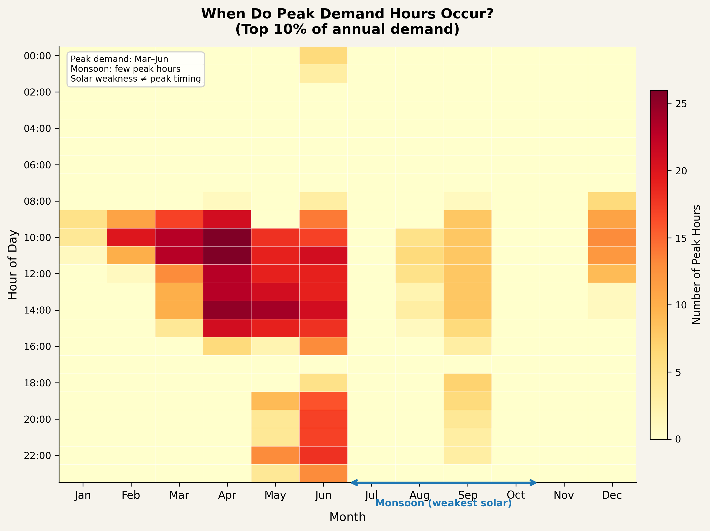
Load-following achieves perfect reliability because India’s electricity demand is structurally aligned with its solar resource: demand peaks during March–June, exactly when pre-monsoon skies produce the year’s strongest solar generation, and drops during the monsoon (July–September), exactly when solar is weakest. The hardest hours for solar (monsoon nights) are precisely when India needs the least power, with demand troughs at 50–60 GW. The fleet’s battery reserves face their lightest demand exactly when the solar resource is at its weakest. The residual shortfall under flat-block dispatch (372 hours across 10 years, 0.4% of all hours under the 3% Bernoulli outage assumption) clusters on winter and monsoon nights predictably: 48.9% on winter nights when Western Disturbances suppress northwest solar for 2–4 consecutive days, 36.3% during monsoon nights, and effectively zero hours during daytime (9 AM–4 PM). These failures are shallow (the fleet never drops to a level that threatens system stability even in its worst hour) and concentrated in periods when electricity demand is just 69–79% of peak. This is the inverse of coal fleet failures, which cluster during summer demand peaks when thermal plants face simultaneous water scarcity, heat-related efficiency losses, and fuel supply stress.
India continues to commit new coal capacity on the assumption that renewables cannot deliver firm power. Yet at plant-gate LCOEs of INR 4.8–5.7/kWh (median INR 5.08/kWh, matching Part 1), every plant in the fleet already undercuts new coal’s all-in delivered range while delivering a fixed 25-year tariff with zero fuel-price risk. The cost of firmness (moving from raw fleet energy to 99.2–100.0% guaranteed delivery) is approximately INR 0.53/kWh, a ~10% premium achieved entirely through smarter dispatch, not additional hardware. Applied symmetrically, inter-state transmission (ISTS) charges of INR 0.50–1.00/kWh (mid 0.75) bring the fleet’s firm flat-block cost to INR 6.11–6.61/kWh delivered (mid 6.36), versus new coal’s bus-bar INR 5.38–6.30/kWh which rises to INR 5.88–7.30/kWh delivered (mid 6.59) once ISTS is added, so the fleet’s all-in delivered midpoint sits INR 0.23/kWh below new coal. Current procurement frameworks require each plant to independently guarantee round-the-clock output, forfeiting the portfolio-level diversification and coordination that make coal fleets themselves reliable. A fleet-level compliance framework, analogous to the NLDC’s existing Security Constrained Economic Dispatch for thermal generation, could unlock firm solar at scale without new infrastructure. What a geographically coordinated fleet of solar with 16 usable hours of storage can deliver, when dispatched as a portfolio rather than as isolated plants, has not been tested in India’s procurement design.
1. Introduction
1.1 The Reliability Question
Solar-plus-storage in India is already cost-competitive with new coal: co-located configurations with 16+ hours of storage are estimated at INR 4.0–4.3/kWh (Chojkiewicz et al., 2025) [8] and SECI’s RTC-IV tender discovered tariffs of INR 5.06–5.07/kWh [21], against new supercritical coal’s first-year INR 5.38–6.30/kWh, yet utilities still committed ~ 11.9 GW of new coal in 2025 alone (Energetica India, 2025) [15]. Solar and battery component costs in India have fallen dramatically. Cost competitiveness alone has not been sufficient. The deeper barrier is reliability credibility: grid planners need to know that a power source can be counted on to deliver every hour, through monsoons, through consecutive cloudy days, through winter nights.
Consider a single co-located plant: 5 GW of solar capacity paired with 17.78 GWh of battery storage (16 GWh usable above 10% SOC floor), sized to deliver 1 GW of firm power around the clock. Even with this generous provisioning (roughly 16 hours of storage at rated output), extended cloudy periods eventually deplete the battery. Consecutive monsoon days, winter Western Disturbances, and pre-monsoon haze can suppress generation for long enough that the median plant delivers its target output in roughly 92% of hours; in the remaining hours, output can collapse to zero. No single location in India has sufficient solar consistency to guarantee round-the-clock power from a finite battery, but no single coal plant guarantees this either.
India’s procurement frameworks have not absorbed this distinction. SECI’s RTC and FDRE tenders require each project to independently meet availability targets: plant-level compliance for what may be a fleet-level problem. The result is plant-level oversizing to meet stringent service obligations: FDRE tariffs have reached INR4.98–8.50/kWh (SECI FDRE Tranches IV–VII, 2024–2026) [13], with the upper tranches well above the INR5.61/kWh we estimate for fleet-level firm delivery (§3.5). Part of this gap reflects FDRE’s genuinely harder product (90% Demand Fulfillment Ratio with designated peak-hour delivery, not flat-block); the bulk reflects plant-level compliance, which forces each project to oversize rather than letting geographic diversity across the fleet substitute for storage. As of early 2026, no fully integrated gigawatt-scale RTC project in India is operating as contracted (SECI, 2024) [3]. The binding question for India’s power sector is therefore not only whether solar-plus-storage is affordable (emerging evidence suggests it can be) but whether it can deliver the fleet-level reliability that makes coal the default choice for capacity adequacy planning. The Central Electricity Authority projects that India will require approximately 307 GW of thermal capacity by 2035 to guarantee supply security (CEA NEP, 2023) [4]. This projection rests on the assumption that renewable energy cannot provide equivalent firm power. This paper tests that assumption.
This continental-fleet analysis is the second of a two-part study. The companion paper (Paliwal, Abhyankar & Phadke, 2026, Part 1: Plant-Level Evidence for Firm Solar in India) [37] shows that a single co-located 5 GW-AC solar + 16 GWh battery plant, identical in architecture to each of the 120 plants modeled here, already meets the Central Electricity Regulatory Commission’s coal-equivalent availability norm (≥85 percent annual NAPAF, ≥90 percent during peak months) at a plant-gate LCOE of INR 5.08/kWh across 10 high-resource Indian states (82 of 100 site-weather-years pass all availability criteria), all of which are drawn from the same 120-site fleet used in this paper. Part 1 closes the plant-level credibility gap against an individual coal unit; this paper closes the fleet-level gap against the coal fleet as a whole.
1.2 The Geographic Diversification Hypothesis
Individual coal plants are normatively rated at 85% Annual Plant Availability Factor (CERC Tariff Regulations, 2024) [17]. Because forced outages across plants are largely independent, India’s coal fleet historically meets system demand in over 99% of hours despite its plant-level availability ceiling: peak monthly fleet-available capacity in FY24 was approximately 88% (CEA Monthly Reports) [38], even as Part 1 finds the actual coal fleet averages only ~ 76% annual PAF against the 85% normative standard [37]. No single coal unit is firm; the fleet is. Geographic aggregation across uncorrelated regimes has been shown to reduce aggregate variability for wind power in Europe and the United States [22, 23]. Coal plant failures are mechanical and random; solar-plus-storage shortfalls are driven by weather. The question is whether weather-driven failures across India’s 3,000 km span are sufficiently uncorrelated to produce the same diversification effect, and whether, combined with coordinated battery dispatch, it can close the gap to firm power.
One qualification, documented in Part 1’s parse of CEA’s daily outage data [37], sharpens rather than weakens this analogy: coal outages combine an idiosyncratic mechanical component (boiler, turbine, and electrical failures), which does diversify across the fleet, with a common-mode component (shared coal logistics, cooling-water stress, and heat waves) which does not: roughly 24.5 GW of thermal capacity was on forced outage on 30 May 2024, the day India met its 250 GW all-time peak. The coal fleet’s diversification benefit is therefore real but partial. The solar-plus-storage fleet analyzed here inverts that structure: its equipment outages are small, granular, and statistically independent across plants, while its weather-driven shortfalls, though regionally correlated, are seasonal, forecastable, and concentrated in low-demand night hours (§3.4). Fleet aggregation therefore has at least as much to work with for solar-plus-storage as it does for coal.
India’s geography is particularly well-suited to this approach. The subcontinent spans approximately 3,000 km north–south and 2,900 km east–west, across tropical, subtropical, and temperate climate zones with three largely independent weather regimes: the northwest (Rajasthan, Gujarat) with India’s strongest solar resource; the northeast (Assam, Tripura) with monsoon patterns largely anti-correlated to the west; and the south (Tamil Nadu, Karnataka) with a rainy season (October–December) offset from the June–September southwest monsoon affecting the rest of India. A geographically distributed fleet inherits these decorrelations automatically. But diversification alone only creates heterogeneity in plant conditions (some plants sun-rich, others depleted) without a mechanism to redistribute energy across them. That mechanism is coordinated battery dispatch.
2. Methodology
The complete methodology, including the full LP formulation, site selection algorithm, and design rationale, is provided in Appendix A. This section summarizes the key elements.
We simulate 120 DC-coupled solar-plus-storage plants (5.0 GW-AC solar, 17.78 GWh nameplate / 16 GWh usable battery each) distributed across 18 Indian states and compare independent and coordinated dispatch strategies for meeting a 100 GW aggregate output target across ten weather years (2015–2024), totaling 87,600 simulated hours spanning El Niño, La Niña, and neutral ENSO phases. We evaluate fleet reliability against both a constant flat-block target (the most demanding test, requiring identical output every hour) and India’s actual hourly demand shape, and examine the relative contributions of geographic diversification and operational coordination.
Data. Hourly solar capacity factors come from NREL’s India dataset [1], covering 157,715 grid cells at ~5 km resolution for ten years (8,760 hours each). Site-level land availability and transmission proximity come from NREL’s companion supply curve dataset [2] (~46,000 cells at 5.76 km resolution). Hourly state-level electricity demand data come from Grid-India (POSOCO/NLDC) [11] (calendar year 2022); for load-following scenarios, national demand is normalized so that the peak equals 100 GW.
Site selection. We select 120 sites using a scoring algorithm that weights developable land area (70%) and transmission proximity (30%), subject to geographic-diversity caps (up to 12 sites per state, with the lower bound of 2 contingent on a state having a candidate block clearing the developable-land threshold). Each site comprises a 2×2 block of adjacent grid cells (~11.5 × 11.5 km). The resulting fleet spans latitudes 9.4°N–35.3°N across 18 states, with the largest concentrations in Rajasthan (36), Gujarat, Assam, J&K, and Tripura (12 each).
Plant configuration. Each plant pairs 5.0 GW-AC of solar PV (7.0 GW-DC at an inverter loading ratio of 1.4) with 17.78 GWh of battery storage behind a 1 GW grid inverter. The DC-coupled architecture allows the full solar array to charge the battery directly without inverter bottlenecks. The 5:1 AC solar-to-output ratio (7:1 at DC level) yields ~19% daily energy surplus over the 24 GWh consumption target at the fleet’s mean 17% capacity factor, accommodating 92% round-trip efficiency losses and below-average solar days. The 16-hour usable (17.78 GWh nameplate) storage duration covers India’s longest winter nights (~13.5 hours) with substantial margin. Battery dispatch is subject to a 10% minimum state-of-charge constraint (standard for LFP chemistry), leaving 16 GWh of usable capacity, and each plant experiences independent forced outages at a 3% per-hour Bernoulli rate, modeled stochastically inside the linear program with a seeded outage mask for reproducibility (Appendix A.3, A.4.2). The fleet’s 120 GW nameplate capacity provides a 20% reserve margin over the 100 GW target.
Dispatch strategies. Under greedy dispatch, each plant operates independently with no coordination or foresight: surplus solar charges the battery; deficits draw from storage; any remaining shortfall is unmet. Under coordinated dispatch, a central fleet operator schedules battery charge and discharge across all plants to minimize aggregate shortfall, analogous to the Security Constrained Economic Dispatch (SCED) that India’s National Load Dispatch Centre already runs for thermal generation (Grid-India, 2022) [11]. We model this using a linear program (LP) with perfect foresight over 8,760 hours (Appendix A, Equations 1–8), which provides an upper bound on what coordination can achieve; real-world implementation would use day-ahead solar forecasts with intraday re-optimization, a standard practice in ISO/RTO markets worldwide. The national formulation contains ~5.3 million decision variables and ~4.2 million constraints, solved using the HiGHS LP solver (Huangfu & Hall, 2018) [6] via CVXPY (Diamond & Boyd, 2016) [5]. Greedy dispatch provides a lower bound on fleet reliability; the perfect-foresight LP provides an upper bound. The gap between them quantifies the value of coordination: reliability gained purely through operational strategy, without additional hardware.
Evaluation scenarios. We test five configurations: a greedy baseline plus four coordinated scenarios spanning two target types and two coordination scopes. Flat-block requires constant 100 GW output every hour, the most demanding test. Load-following tracks India’s actual hourly demand shape (ranging ~50.5–100 GW). National coordination optimizes all 120 plants jointly; state-level coordination runs 18 independent LPs, one per state. The primary metric is hourly reliability: the fraction of 8,760 hours in which aggregate output meets or exceeds the target. We also report worst-hour output, energy curtailment, and coefficient of variation. All five scenarios are run independently for each of the ten weather years, spanning El Niño, La Niña, and neutral ENSO phases.
3. Results
We present results in stages, building from the single-plant baseline to fleet-level outcomes. Section 3.1 describes the geographic distribution of sites. Section 3.2 establishes the single-plant performance limit. Section 3.3 presents the headline result (fleet aggregation and coordinated dispatch under the flat-block target) together with the physical mechanisms that explain the gains. Section 3.4 validates robustness across ten weather years (2015–2024) and analyzes residual failures. Section 3.5 extends the analysis to load-following dispatch and presents system costs. State-level reliability analysis is provided in Supplementary Table S1. Individual plant compliance against India’s RTC-IV framework is reported in Supplementary Section S2.
3.1 Site Selection and Geographic Distribution
The site selection algorithm placed 120 plants across 18 states, from Kerala in the south to Jammu & Kashmir in the north and from Gujarat in the west to Tripura in the east. This geographic spread, spanning nearly all of India’s mainland, is the architectural foundation of the system: sites experience distinct monsoon regimes, diurnal irradiance patterns, and seasonal weather cycles (Figure 1).
Notably, that score (70% developable land, 30% transmission proximity) does not reward solar resource quality or weather diversity; it ranks candidates only by deployable land and grid access. The 2–12 per-state cap is the implicit diversification instrument: because Indian state boundaries broadly track the country’s climatic regions, capping any single state at 12 plants forces the remaining slots into states with distinct weather. The cap binds first in Rajasthan (highest-scored blocks), then in Gujarat and J&K (also northwest), then spills into the high-land-availability northeastern belt (Assam, Tripura, Arunachal Pradesh), which is climatologically uncorrelated with the northwest (Figure 3, ρ ≈ 0.01–0.05). Central-Indian states (UP, Bihar, MP, Odisha, Jharkhand) score poorly on the 30 km² contiguous-block test once Rajasthan-grade land is unavailable, which is why the fleet appears bimodal, clustered in the northwest and northeast, rather than uniformly spread. This bimodality is the experiment, not an accident: those two clusters are India’s two most weakly correlated weather regimes. Those northeastern sites have materially weaker solar resource than the western desert. The cost penalty of weaker resource is modest: solar modules account for roughly 25–30% of total project cost (Appendix B), and increasing the inverter loading ratio can largely compensate for lower irradiance. Part 1 of this study (Paliwal, Abhyankar, Phadke) [37] shows that a single such site, in any of ten high-resource states evaluated independently, already meets coal’s 85% NAPAF norm, so the fleet considered here is built from plants each of which is already coal-equivalent on its own.
120 plants across 18 states, sited for resource and diversity
Plant locations by region · every plant 5.0 GW-AC solar + 17.78 GWh nameplate battery, 1 GW firm output
UC BERKELEY ANALYSIS · AUGUST 2026
View the data table
120 plants aggregated to 18 states; marker size on the map is constant and only shade varies. Extent lon 67–98, lat 6–38, equal aspect. Every plant is identical — the same solar and battery build against the same 1 GW target — so marker size carries nothing and only shade varies.
| State | Region | Plants | Mean cf | Min cf | Max cf |
|---|---|---|---|---|---|
| Rajasthan | Northwest | 36 | 0.1769 | 0.1723 | 0.1792 |
| Assam | Northeast | 12 | 0.1517 | 0.1444 | 0.1575 |
| Gujarat | Northwest | 12 | 0.1787 | 0.1772 | 0.1811 |
| Jammu & Kashmir | Northwest | 12 | 0.2053 | 0.2024 | 0.2096 |
| Tripura | Northeast | 12 | 0.1545 | 0.1541 | 0.1552 |
| Arunachal Pradesh | Northeast | 7 | 0.1439 | 0.1399 | 0.1466 |
| Kerala | Southwest | 6 | 0.1726 | 0.1717 | 0.1739 |
| Andhra Pradesh | Southeast | 5 | 0.1704 | 0.1689 | 0.1725 |
| Karnataka | Southwest | 5 | 0.171 | 0.1689 | 0.1735 |
| Chhattisgarh | Southwest | 3 | 0.1674 | 0.1667 | 0.1681 |
| Haryana | Northwest | 2 | 0.1659 | 0.1655 | 0.1663 |
| Maharashtra | Southwest | 2 | 0.1678 | 0.1677 | 0.1678 |
| Madhya Pradesh | Northwest | 1 | 0.1685 | 0.1685 | 0.1685 |
| Meghalaya | Northeast | 1 | 0.1524 | 0.1524 | 0.1524 |
| Tamil Nadu | Southeast | 1 | 0.1746 | 0.1746 | 0.1746 |
| Telangana | Southeast | 1 | 0.1668 | 0.1668 | 0.1668 |
| Uttarakhand | Northwest | 1 | 0.1656 | 0.1656 | 0.1656 |
| West Bengal | Northeast | 1 | 0.1514 | 0.1514 | 0.1514 |
| All states | Northwest 64 · Southwest 16 · Southeast 7 · Northeast 33 | 120 | 0.1713 | 0.1399 | 0.2096 |
3.2 The Single-Plant Constraint
Before examining fleet behavior, it is instructive to understand the performance limits of an individual plant: 5.0 GW-AC of solar (7.0 GW-DC) paired with 17.78 GWh of battery storage (16 GWh usable), targeting 1 GW of constant output. Under independent (greedy) dispatch each plant charges its battery by day and discharges it overnight to hold 1 GW. The problem emerges during consecutive cloudy days: with reduced solar input, the battery cannot fully recharge, and state of charge progressively declines until the plant can no longer meet its target.
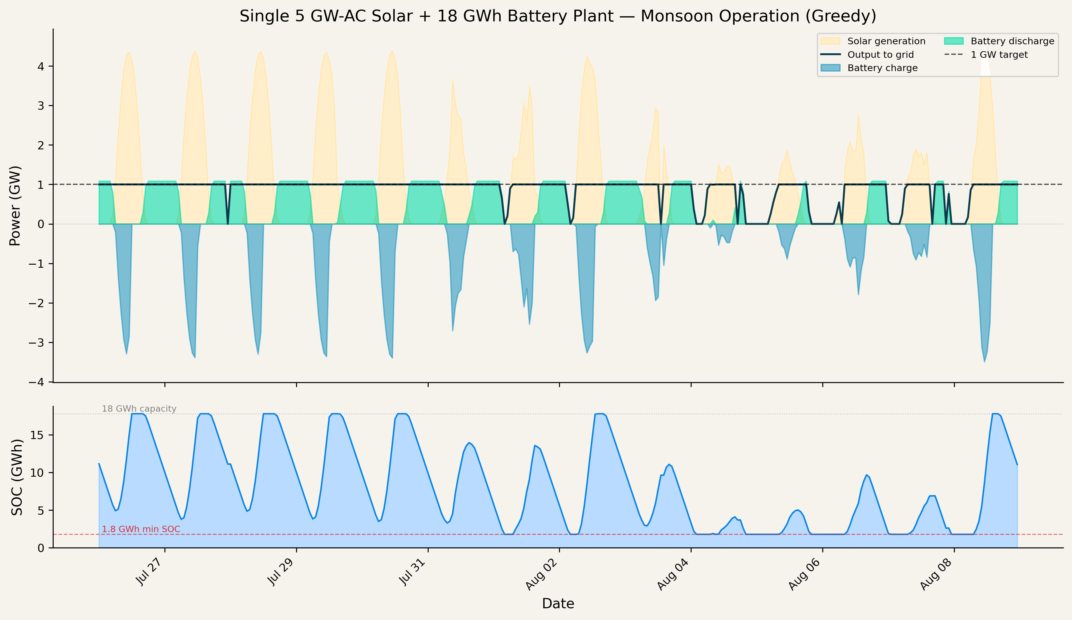
Across the ten weather years (2015–2024), individual plant performance under greedy dispatch varies widely. The best plants (Jammu & Kashmir, Rajasthan) deliver ≥ 1 GW output in about 94% of hours, while the worst (Arunachal Pradesh) manage only 77%. Across all 120 plants, the median hourly reliability (the fraction of hours delivering the full 1 GW target) is 92.0%, with 704 shortfall hours per year. But this number masks the severity of failures: when a plant falls short, average shortfall depth is 83% of the target, output drops to zero in the worst hours, and shortfalls can last up to 40 consecutive hours. The median plant (Rajasthan) swings between full output and zero across the year: when the battery depletes, output drops to nothing. Figure 2 illustrates the median plant’s operation during a two-week monsoon period: as consecutive cloudy days deplete the battery, output repeatedly falls short of the 1 GW target. No single location in India has sufficient solar consistency to guarantee round-the-clock output from a finitely-sized battery. Nevertheless, the 5:1 AC DC-coupled configuration (7:1 at DC level) already transforms each plant from a variable solar generator into a near-baseload product, even after accounting for the 10% minimum SOC constraint and 3% per-plant per-hour Bernoulli forced outage. At an estimated INR5.08/kWh (Appendix B), this single-plant product is already below new supercritical coal (INR5.38–6.30/kWh; Energetica India, 2025) [15], before any fleet-level benefits are considered.
Figure 3
UC BERKELEY ANALYSIS · AUGUST 2026
3.3 Fleet Performance: Aggregation, Coordination, and Mechanisms
Stage 1: Geographic aggregation (greedy dispatch). When the same 120 plants are simply summed (each still operating independently, exactly as in Section 3.2), the effect of geographic diversity is immediate. A single plant’s worst hour produces zero output. The fleet’s worst hour still delivers 27.3 GW. No coordination, no optimization, just arithmetic aggregation across 18 states, and the catastrophic single-plant failure mode disappears entirely. The fleet meets the full 100 GW target in 84.0–88.5% of hours, with a mean output of ~110 GW and total energy delivery of 965 TWh per year (10-year greedy mean).
The fleet’s 86.0% hourly reliability appears comparable to the median plant’s 92.0%, even slightly worse, because the 100 GW aggregate target is harder to hit perfectly than a single plant’s 1 GW target. But reliability percentages mask a qualitative transformation in the character of failures. When a single plant fails, output collapses to zero: shortfall depth averages 83% of the target, and failures last up to 40 consecutive hours. The fleet’s shortfalls are shallow: average depth is just 12%, and worst-hour output never falls below 27.3 GW (27% of target). Normalized energy-not-served drops from 6.6% to 1.6%, and the coefficient of variation of hourly output halves from 25.7% to 9.5%. This is the diversification dividend: geographic decorrelation transforms deep, catastrophic single-plant failures into mild fleet-level dips.
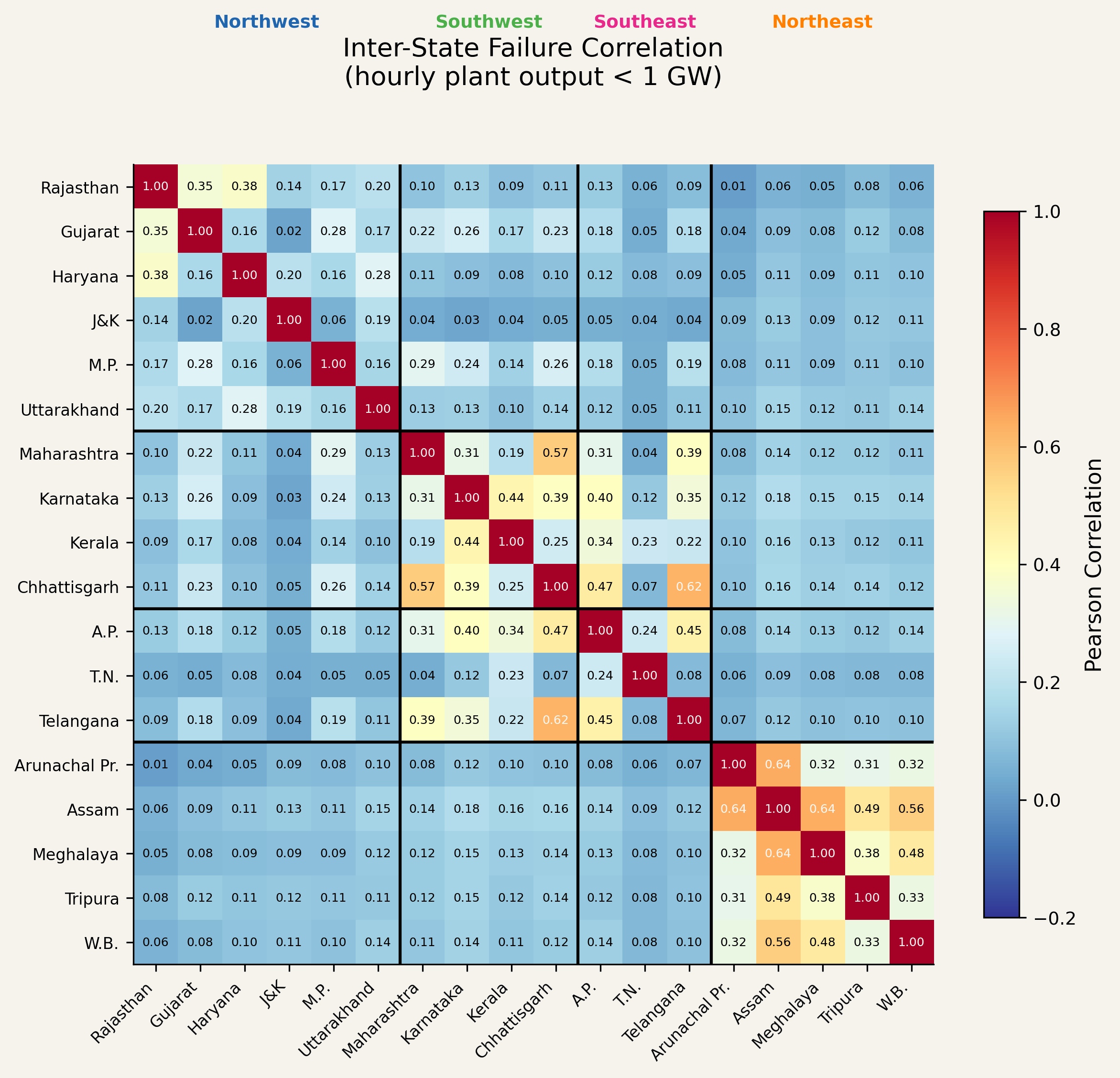
Why aggregation works: spatial decorrelation of failures. We define a plant-level failure as any hour in which a plant’s output falls below its 1 GW target. Figure 3 shows the inter-state correlation of these failure events under greedy dispatch. The pattern maps directly onto geographic distance. States within the same region share correlated weather and therefore correlated failures: Rajasthan and Gujarat (both in the northwest, ~500 km apart) show correlation of 0.5–0.8, as do the northeastern states Assam, Arunachal Pradesh, and Tripura (~200–400 km apart). States across regions, separated by 1,500–2,500 km, are nearly uncorrelated: Rajasthan and Assam (0.01–0.05), Gujarat and Tripura (0.02–0.06), Jammu & Kashmir and Kerala (0.03–0.08). The southern states (Karnataka, Kerala, Tamil Nadu) show moderate correlation with each other but low correlation with both the northwest and northeast clusters. This geographic decorrelation is what makes fleet-level aggregation effective: the fleet spans enough of the subcontinent that no single weather system can suppress output everywhere simultaneously.
Figure 4
UC BERKELEY ANALYSIS · AUGUST 2026
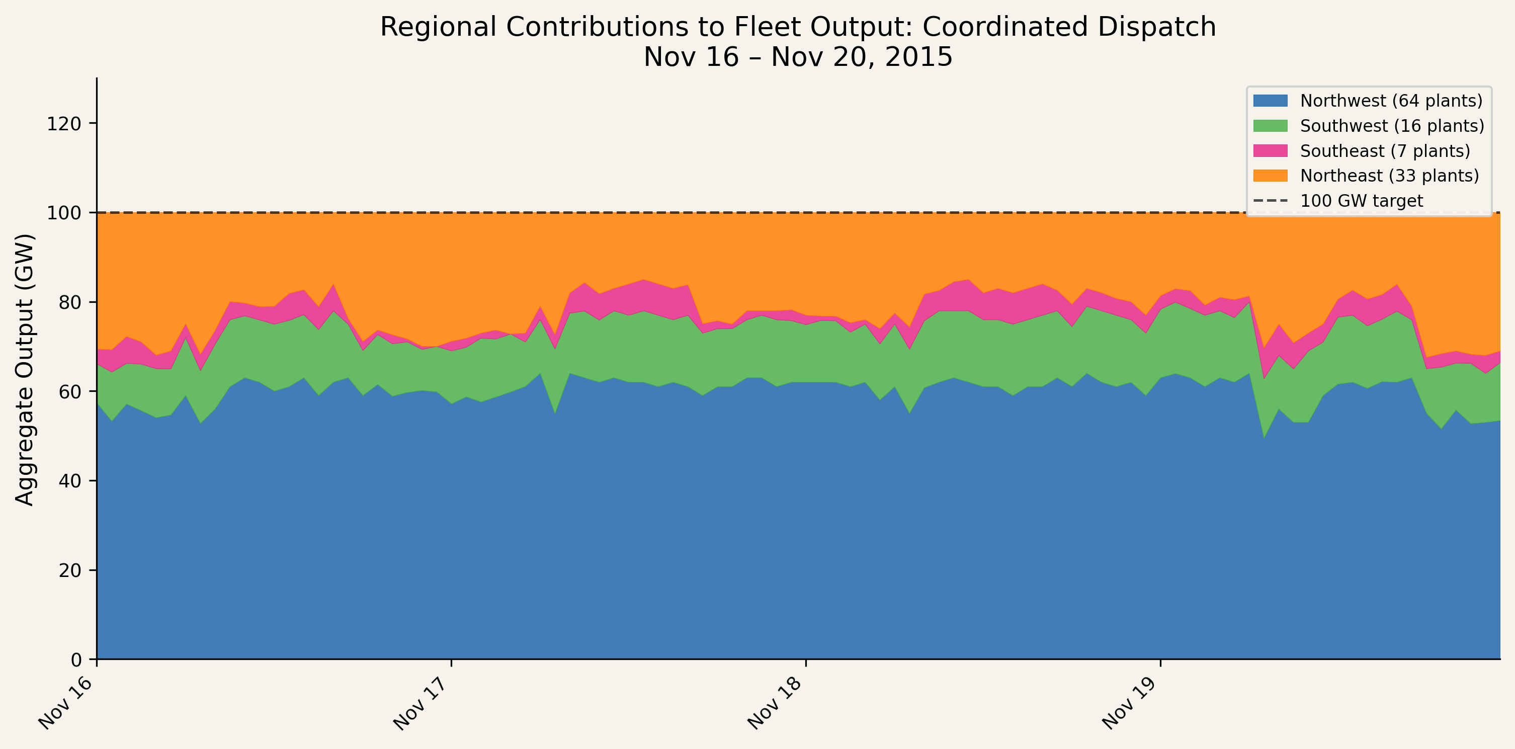
Regional compensation in action. When one region experiences reduced solar output, other regions compensate, maintaining aggregate fleet output at the 100 GW target. Figure 4 illustrates this during November 16–20, 2015, when the northeast monsoon suppressed solar generation across southeast India. During this period, the Southeast region’s output dropped 35% below its annual mean, and the Northeast declined 8%, as cloud cover from the retreating monsoon and early winter weather moved across eastern and southern India. Simultaneously, the Northwest, experiencing clear post-monsoon skies typical of November in Rajasthan and Gujarat, surged 7% above its annual mean, expanding from its normal 56 GW contribution to nearly 60 GW. The result: the fleet delivered exactly 100 GW in every hour of the four-day period, with zero shortfall, despite a significant regional weather disruption. As weather fronts move across the subcontinent, regional shares shift (Northwest dominance gives way to Southeast and Northeast contributions and vice versa), yet the aggregate remains pinned at the target. This temporal complementarity across regions is the physical mechanism through which spatial diversity converts variable solar into firm power.
Figure 5
UC BERKELEY ANALYSIS · AUGUST 2026
Stage 2: Coordinated fleet dispatch (optimized). Centrally coordinated dispatch (where a system operator schedules battery charge and discharge across all 120 plants based on solar forecasts) raises reliability against the 100 GW flat-block target from ~86% to 99.2–100.0% under the 3% Bernoulli outage assumption, compressing the shortfall by an order of magnitude. The worst-hour floor rises from 27.3 GW to 32.5 GW under coordination, and the CV of hourly output drops from 9.5% to 1.5% (Figure 5): the optimized trace is nearly indistinguishable from a flat line at 100 GW. The residual coordinated shortfalls are rarer but deeper than greedy’s (mean depth 17% of target vs 12%): coordination eliminates the shallow, avoidable dips, leaving only the hard core of prolonged multi-day weather events.
| Metric | Single Plant (median) | Greedy Fleet | Coordinated Fleet |
|---|---|---|---|
| Reliability (%) | 92.0 (at 1 GW) | 86.0 (at 100 GW) | 99.6 (at 100 GW) |
| Hours ≥ 95 GW (%) | n/a | 90.5 | 99.7 |
| Shortfall hours | 704 | 1223 | 37 |
| Shortfall depth (%) | 83 | 12 | 17 |
| Worst-hour output | 0 GW (0%) | 27.3 GW | 32.5 GW |
| Longest shortfall (hrs) | 40 | 17 | 15 |
| Normalized ENS (%) | 6.6 | 1.6 | 0.07 |
| Output CV (%) | 25.7 | 9.5 | 1.5 |
| Energy delivered | n/a | 965 TWh | 876 TWh |
Ranges shown reflect 3% per-plant per-hour Bernoulli forced outage, modeled with a seeded mask inside the LP (Appendix A.4.2).
See Figure 1 above.
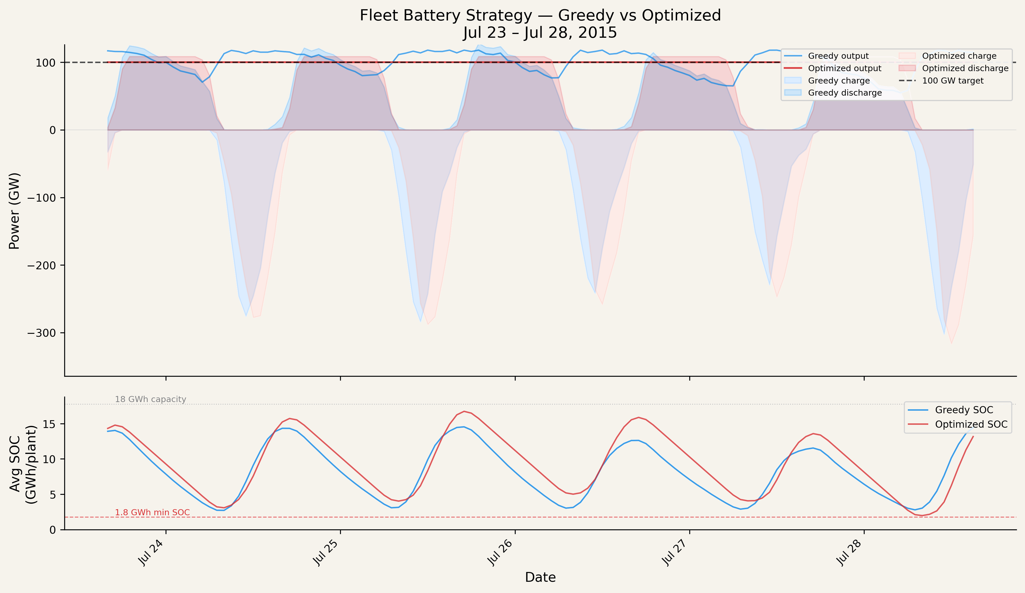
How coordination works: differentiated battery management. The reliability improvement from coordination (86.0% to 99.6%) requires no additional hardware, only smarter battery management. Under greedy dispatch, all batteries follow essentially the same cycle: charge during the day, discharge at night, respecting the 10% minimum SOC floor. When several consecutive cloudy days hit a region, every plant in that region depletes to its minimum on the same schedule, causing regional fleet failure. The 3% Bernoulli per-hour outage removes on expectation ~3.6 plants per hour (with a variable number in any given hour drawn from the Bernoulli mask), compounding the uniform-depletion problem in plants that happen to be out during a regional stress event. The optimizer breaks this uniform depletion pattern by differentiating battery behavior across plants. Since the fleet only needs to deliver 100 GW from 120 plants (minus on expectation ~3.6 plants from the Bernoulli outage draw), the optimizer throttles 15–25 operational plants per hour during high-solar periods, reducing their grid output below 1 GW and diverting the freed solar energy into their batteries. Other plants with above-average solar compensate by delivering their full 1 GW to maintain the aggregate target. With perfect foresight, the optimizer selectively builds reserves at plants that will face cloudy conditions in coming hours or days.
Figure 6 compares fleet-average battery state of charge between greedy and optimized dispatch during a monsoon week: the optimizer maintains consistently higher battery reserves before evening periods, preventing the output collapses that occur when each plant independently drains its battery.
Figure 6
UC BERKELEY ANALYSIS · AUGUST 2026
3.4 Multi-Year Robustness and Failure Analysis
The results presented thus far use a single weather year (2015). We repeat the analysis across all ten available weather years (2015–2024), encompassing 87,600 simulated hours spanning El Niño, La Niña, and neutral ENSO phases.
Optimized flat-block reliability ranges 99.2–100.0% under the 3% Bernoulli outage assumption, with the worst year (2020) producing 67 shortfall hours out of 8,760; 2016 and 2018 had zero shortfall. Figure 7 summarizes these results.
99.2–100% reliability, in every one of ten weather years
Share of hours at the 100 GW target by weather year and dispatch mode · 2015–2024 · % of hours
UC BERKELEY ANALYSIS · AUGUST 2026
View the data table
All ten columns, including the eight the published figure omits. Rel% is the share of the 8,760 hours meeting the 100 GW target; CV% is the coefficient of variation of fleet output and is a different unit, so it is drawn on its own panel. Reference line 99.2% = the minimum of the optimized flat-block series. Axis limits 0–103.
| Weather year | Greedy Rel% | Greedy CV% | Nat. Flat-Block Rel% | Nat. Flat-Block CV% | Nat. Load-Follow Rel% | Nat. Load-Follow CV% | State Flat-Block Rel% | State Flat-Block CV% | State Load-Follow Rel% | State Load-Follow CV% |
|---|---|---|---|---|---|---|---|---|---|---|
| 2015 | 87.30 | 9.31 | 99.30 | 1.58 | 100.00 | 10.94 | 35.50 | 4.78 | 0.50 | 12.43 |
| 2016 | 88.50 | 8.01 | 100.00 | 0.57 | 100.00 | 10.94 | 37.80 | 3.75 | 0.60 | 12.44 |
| 2017 | 86.50 | 9.42 | 99.80 | 0.97 | 100.00 | 10.94 | 35.70 | 4.59 | 0.50 | 12.57 |
| 2018 | 87.30 | 9.12 | 100.00 | 0.57 | 100.00 | 10.94 | 36.80 | 4.16 | 0.50 | 12.41 |
| 2019 | 84.00 | 10.06 | 99.60 | 1.25 | 100.00 | 10.95 | 34.30 | 5.58 | 0.40 | 12.60 |
| 2020 | 84.10 | 10.36 | 99.20 | 1.65 | 100.00 | 10.94 | 34.20 | 5.42 | 0.40 | 12.41 |
| 2021 | 85.50 | 9.75 | 99.20 | 1.96 | 100.00 | 10.94 | 34.70 | 5.13 | 0.40 | 12.44 |
| 2022 | 85.30 | 9.48 | 99.50 | 1.45 | 100.00 | 10.94 | 34.00 | 5.03 | 0.50 | 12.38 |
| 2023 | 87.20 | 9.27 | 99.50 | 1.96 | 100.00 | 10.94 | 36.10 | 4.49 | 0.50 | 12.49 |
| 2024 | 84.50 | 10.10 | 99.60 | 2.26 | 100.00 | 10.94 | 33.40 | 5.11 | 0.50 | 12.45 |
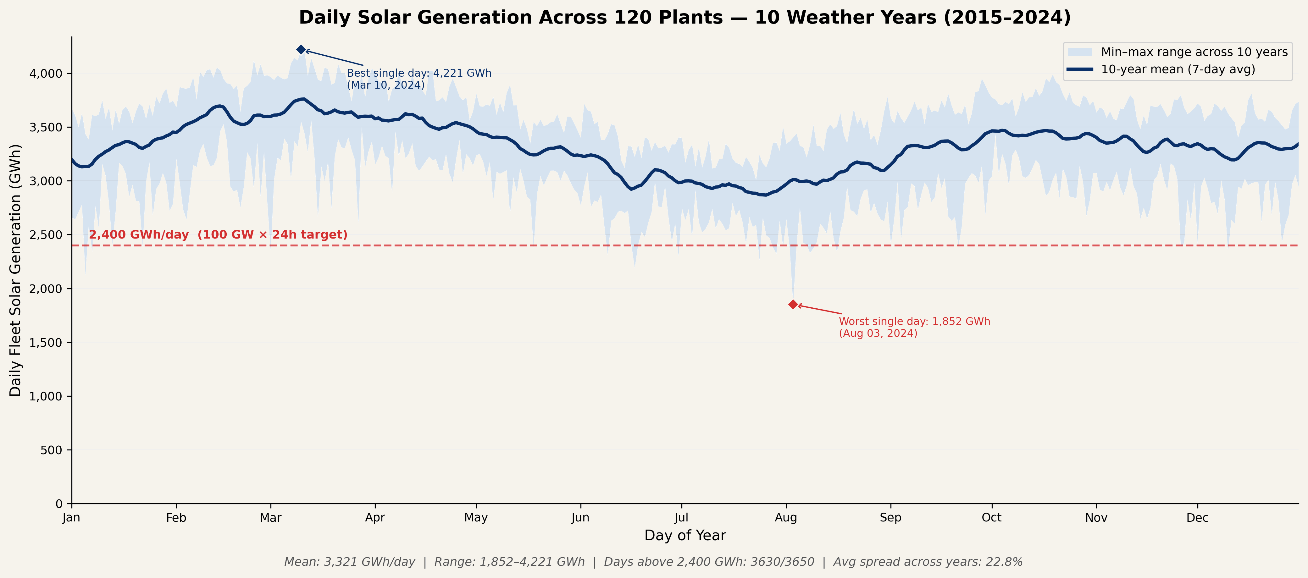
Why reliability is so stable: India’s solar generation has no “winter.” In higher-latitude countries like Germany or the UK, the worst winter month produces only 15–20% of the best summer month’s solar output (Shaner et al., 2018) [23], meaning some years with harsher winters would see dramatically worse reliability than others, and batteries alone cannot bridge a multi-month seasonal deficit. India’s tropical and subtropical latitude (8°N–37°N) eliminates this problem. The 120-plant fleet generates an average of ~3,321 GWh per day, and even in the worst solar month (July, monsoon peak), daily generation is ~3,000 GWh, 80% of the best month (March). Annual gross totals range from ~1,195 TWh to ~1,237 TWh across the decade, a spread of only ~3.5%. Because every year presents roughly the same daily recharge challenge to the batteries (no year has a structurally deeper trough than another), reliability barely varies from one year to the next. The system faces only a daily intermittency problem (bridging nighttime), not a seasonal one, which is why 18 hours of battery storage per plant is sufficient.
Figure 8 visualizes this consistency across the full decade. The bold line shows the 10-year mean daily generation (7-day rolling average), while the shaded band shows the full min–max range across all years. The fleet produces between 1,852 GWh (a single anomalous monsoon day) and 4,221 GWh, yet the mean trace barely deviates from 3,321 GWh outside the monsoon trough.
Figure 8
UC BERKELEY ANALYSIS · AUGUST 2026
Temporal distribution of shortfall. The 372 total shortfall hours across 10 years of optimized flat-block dispatch under the 3% Bernoulli outage assumption fall into two failure modes (Figure 9). Winter nights (November–January) account for ~ 182 hours (48.9%), driven by Western Disturbances suppressing Northwest solar. Monsoon nights (July–September) account for ~ 135 hours (36.3%), driven by widespread cloud cover. The remaining ~ 55 hours (14.8%) are scattered across shoulder months, where forced outages push already-marginal hours below target. All but two of the 372 shortfall hours occur between 17:00 and 08:00 (only 2 isolated hours fall at 09:00), with effectively zero shortfall during daylight: the binding constraint is always overnight battery depletion, never insufficient instantaneous solar.
Shortfalls cluster on winter and monsoon nights, and vanish by day
Distribution of shortfall hours by month and hour of day · optimized flat-block dispatch · 2015–2024
UC BERKELEY ANALYSIS · AUGUST 2026
View the data table
Counts of hours with any unmet demand, ten weather years. The year × month grid prints whole; the 24 × 12 hour-of-day grid is aggregated into the 17:00–08:00 window and its complement, and the per-hour rail is the column sum of that grid. Correction: 371 of 373 shortfall hours fall in that window — not all 373, as the published figure states. Worst single hour 67.51 GW.
| Month | 2015 | 2016 | 2017 | 2018 | 2019 | 2020 | 2021 | 2022 | 2023 | 2024 | Total hours | Severity (GWh) | 17:00–08:00 | Daylight hours |
|---|---|---|---|---|---|---|---|---|---|---|---|---|---|---|
| Jan | 0 | 0 | 0 | 0 | 0 | 37 | 0 | 42 | 0 | 0 | 79 | 1,407.2 | 77 | 2 |
| Feb | 0 | 0 | 0 | 0 | 0 | 0 | 0 | 0 | 0 | 0 | 0 | 0.0 | 0 | 0 |
| Mar | 11 | 0 | 0 | 0 | 0 | 5 | 0 | 0 | 0 | 0 | 16 | 146.7 | 16 | 0 |
| Apr | 0 | 0 | 0 | 0 | 0 | 0 | 0 | 0 | 0 | 0 | 0 | 0.0 | 0 | 0 |
| May | 0 | 0 | 0 | 0 | 0 | 0 | 4 | 0 | 0 | 0 | 4 | 40.4 | 4 | 0 |
| Jun | 14 | 0 | 0 | 0 | 0 | 0 | 0 | 0 | 20 | 0 | 34 | 660.5 | 34 | 0 |
| Jul | 1 | 0 | 0 | 0 | 0 | 0 | 25 | 0 | 0 | 0 | 26 | 602.9 | 26 | 0 |
| Aug | 6 | 0 | 0 | 0 | 8 | 21 | 4 | 0 | 0 | 38 | 77 | 1,582.5 | 77 | 0 |
| Sep | 28 | 0 | 0 | 0 | 0 | 4 | 0 | 0 | 0 | 0 | 32 | 488.1 | 32 | 0 |
| Oct | 0 | 0 | 0 | 0 | 1 | 0 | 0 | 0 | 0 | 0 | 1 | 0.8 | 1 | 0 |
| Nov | 0 | 0 | 0 | 0 | 26 | 0 | 0 | 0 | 24 | 0 | 50 | 785.7 | 50 | 0 |
| Dec | 0 | 0 | 20 | 1 | 0 | 0 | 33 | 0 | 0 | 0 | 54 | 767.9 | 54 | 0 |
| All months | 60 | 0 | 20 | 1 | 35 | 67 | 66 | 42 | 44 | 38 | 373 | 6,482.6 | 371 | 2 |
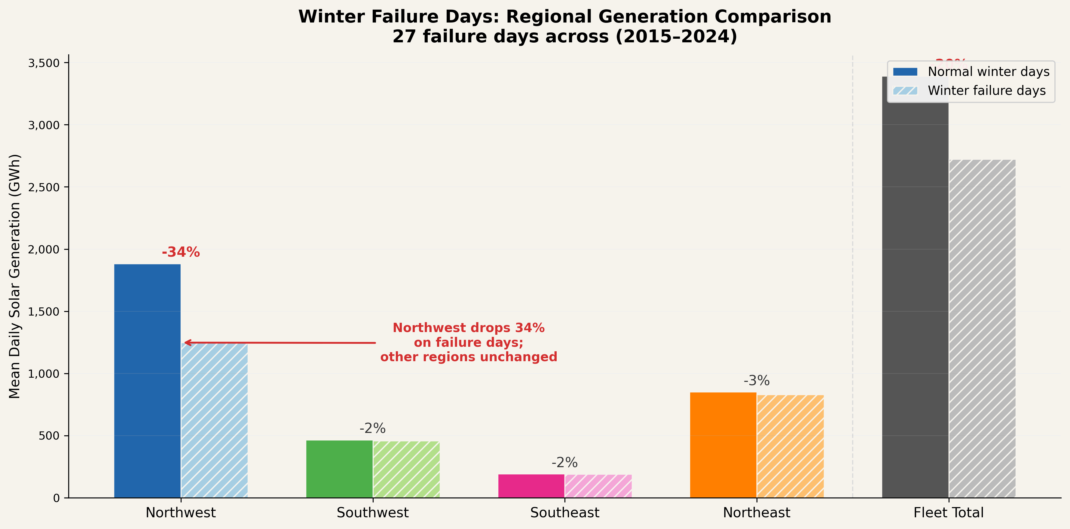
Winter failures: a Northwest-driven phenomenon. The winter shortfall hours (roughly half the total) are not scattered randomly across the season; they cluster into 9 distinct multi-day weather events spanning the decade. We examined regional solar generation on these 26 failure days compared to normal winter days. The pattern is sharply regional: averaged across all failure days, NW generation (64 plants) drops 34% while other regions decline less than 1% (Figure 10). Cross-referencing with India Meteorological Department (IMD) records confirmed Western Disturbance passages as the common cause across all 9 events (IMD, 2015–2024) [25].
The 34% average, however, blends two populations. On the 20 days when a Western Disturbance is actively suppressing NW solar, the drop averages 44% (worst: 70%, just 550 GWh vs the 1,842 GWh winter norm). On the remaining 6 failure days, NW solar has largely recovered, but batteries are still depleted from prior days. These recovery days fail not because of that day’s weather but because the battery needs a full clear day to recharge.
Figure 10
UC BERKELEY ANALYSIS · AUGUST 2026
A live exposure for India’s existing ISTS solar fleet. Rajasthan and Gujarat together host roughly 70% of India’s commissioned ISTS-connected utility-scale solar (MNRE, 2025) [39], and most SECI/NTPC inter-state RTC and FDRE awards to date have landed in these two states [7, 13]. The 35–70% NW solar collapses documented above therefore stress not only the geographically distributed fleet modeled here, but the much less diversified existing ISTS portfolio. A fleet-level compliance regime that explicitly values non-NW capacity for winter-night firmness, rather than awarding solely on lowest plant-gate tariff, would internalize this exposure ex ante.
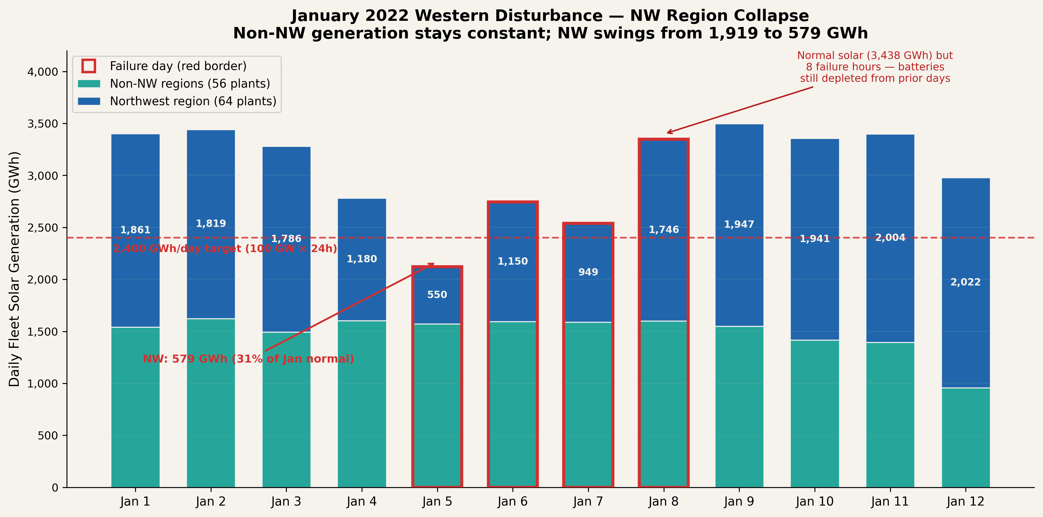
The failures follow a characteristic multi-day sequence. In two-thirds of events, the day before the first shortfall already shows NW generation 24–38% below normal, partially draining battery reserves without yet triggering failure. The WD then fully suppresses NW solar for 1–2 days, pushing batteries to the 10% SOC floor. By the final day, NW solar has recovered but batteries remain depleted; shortfall continues despite adequate sunshine. Short winter daylight (~10.5 hours at 28–35°N) limits the recharging window throughout.
January 5–8, 2022 illustrates all three phases (Figure 11). January 4 (the pre-depletion day): NW dips to 1,180 GWh, no shortfall, but batteries begin drawing down. January 5: NW crashes to 550 GWh (70% below normal) as the WD arrives. January 6–7: NW solar partially recovers (NW-only totals of 1,150 and 949 GWh; fleet totals 2,744 and 2,538 GWh) but batteries are depleted, with 10 and 13 shortfall hours. January 8: NW solar returns to 1,746 GWh (near-normal), yet 8 shortfall hours persist as batteries recharge. Non-NW regions hold steady at ~1,600 GWh/day throughout; the 56 non-NW plants operate near maximum but structurally cannot cover the 100 GW target alone.
Figure 11
UC BERKELEY ANALYSIS · AUGUST 2026
Monsoon failures: multi-day depletion, not single-day collapse. Monsoon failures are rarer than winter ones (~ 135 hours vs ~ 182) and cluster into just 5 events across the decade. Unlike winter, where a single region (the Northwest) collapses while others hold, monsoon suppression is widespread: cloud cover depresses generation across multiple regions simultaneously, leaving fewer compensating sources. But the binding constraint is not any single day’s generation. The battery can bridge one low day using reserves from prior days. Failures require 2–5 consecutive days of depressed generation to progressively drain batteries past recovery.
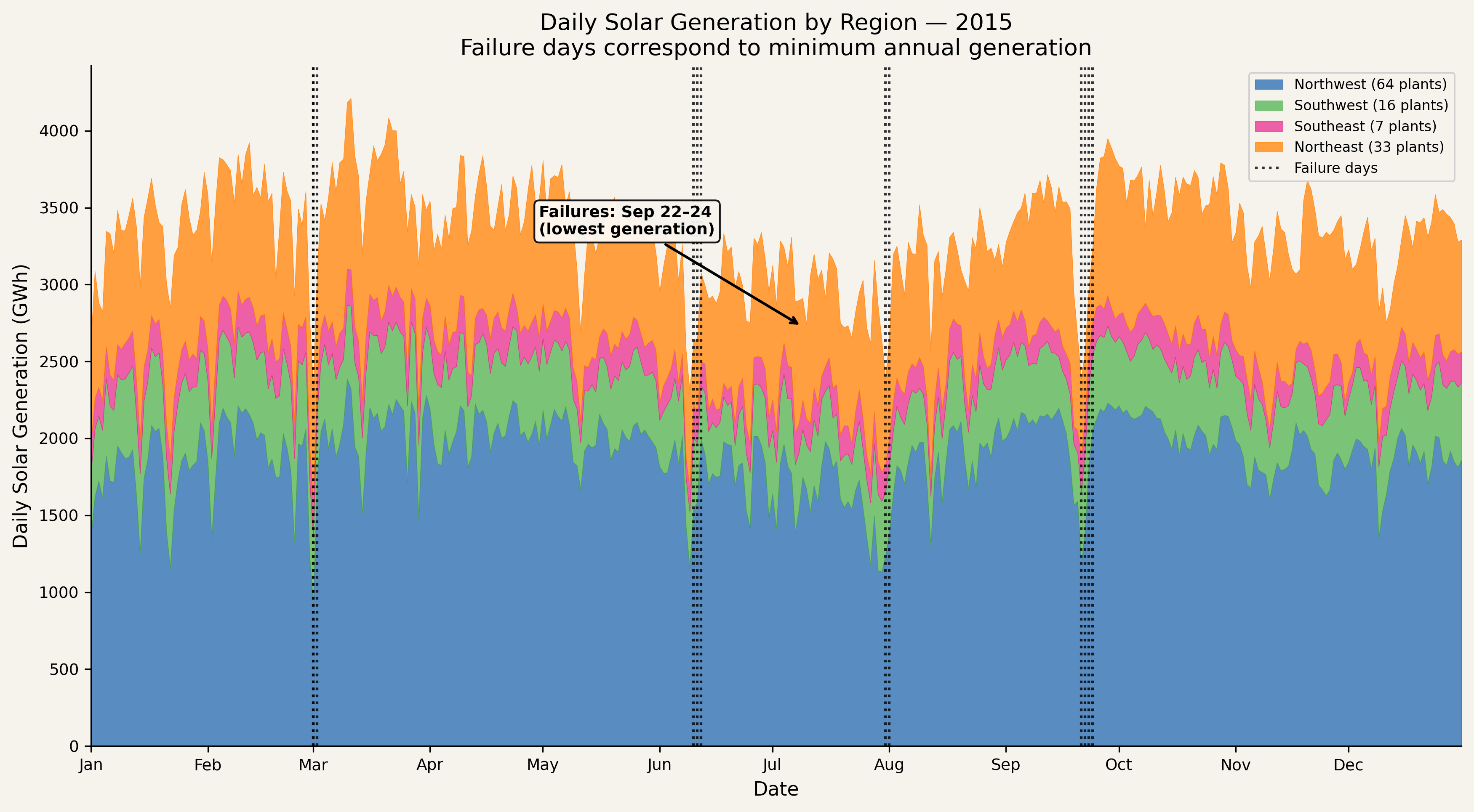
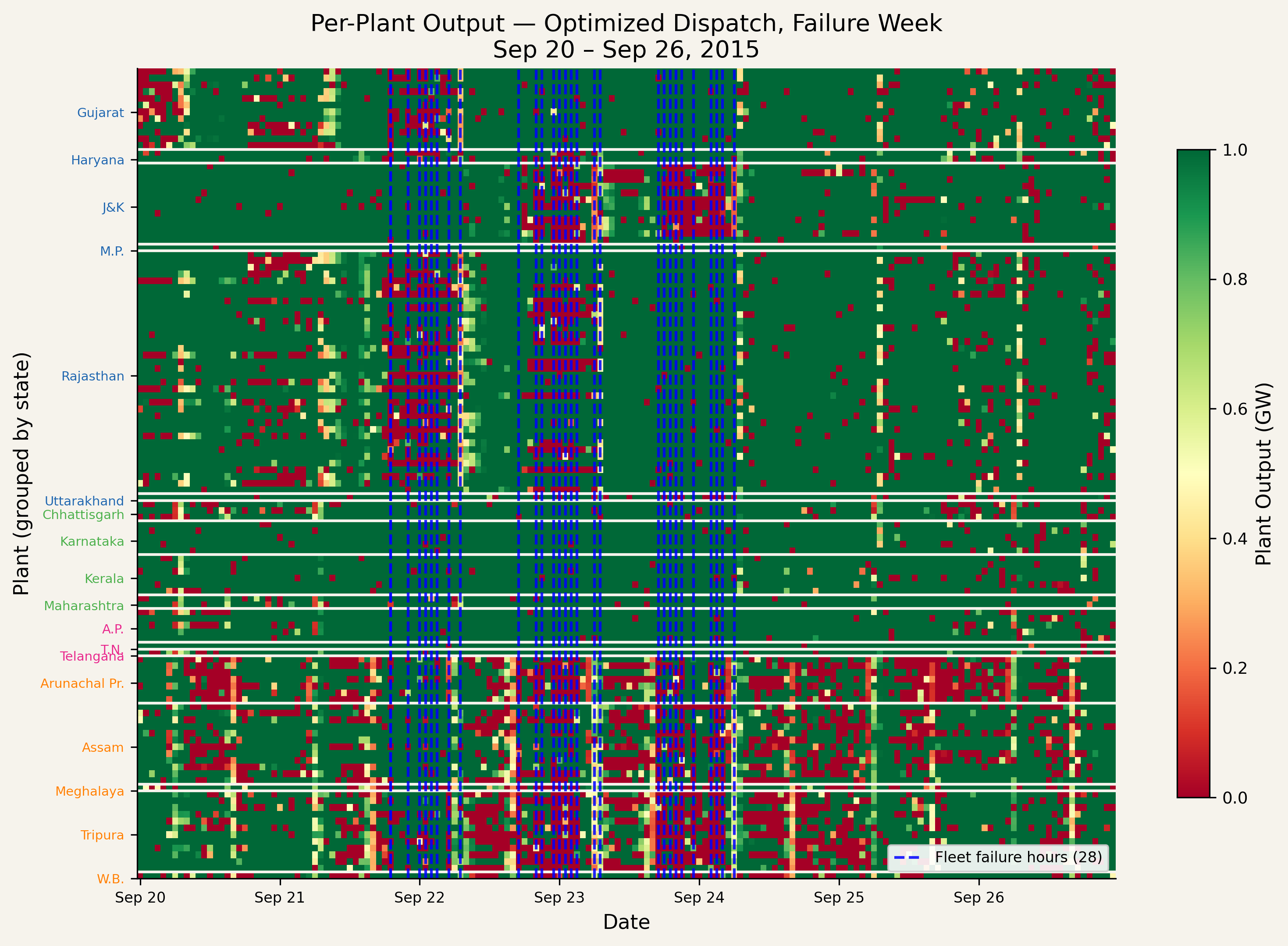
The 2015 reference year illustrates this mechanism: 28 of its 60 failure hours cluster in September 21–24 (the rest spread across the shoulder months, roughly 11 hours in March, 14 in June, and 7 scattered across July–August). September 21–23 had generation at the 1st–5th percentile, progressively depleting battery reserves across the fleet. September 24 had normal generation (66th percentile) but still failed: batteries were already at the 10% SOC floor from the prior three days and needed a full day of recharging before they could bridge the next night. Figure 12 shows daily generation by region across 2015: the failure days sit at the annual floor, the only period when all four regional contributions simultaneously compress. Figure 13 confirms this at the plant level: during these hours, output collapses across nearly every state simultaneously.
Figure 12
UC BERKELEY ANALYSIS · AUGUST 2026
Figure 13
UC BERKELEY ANALYSIS · AUGUST 2026
3.5 Load-Following Dispatch and System Cost
The flat 100 GW target is the most demanding test: it requires peak output every hour of the year. In practice, electricity demand varies throughout the day and across seasons. We use India’s actual hourly demand shape (Grid-India/POSOCO, calendar year 2022) [11], normalized so that the peak equals 100 GW. The resulting target curve ranges from approximately 50.5 GW (monsoon nighttime troughs) to 100 GW (summer afternoon peaks), with a mean of 80.3 GW.
When the optimizer tracks this demand curve instead of the flat 100 GW target, it achieves near-perfect reliability across all 8,760 hours in the 2015 reference year: residual shortfall well under 0.1% of hours, compared to ~ 0.4% of hours under flat-block, even with the 10% minimum SOC constraint and 3% per-plant per-hour Bernoulli forced outage. This improvement reflects a structural alignment between India’s demand and solar resource: demand peaks in March–June, when pre-monsoon skies produce the strongest solar generation, and is lowest during the monsoon months (July–September), precisely when solar output is weakest (Figure 14). The monsoon months that cause the residual flat-block shortfalls are exactly the months where the load-following target drops to 50–60 GW, well within what the fleet can deliver even under cloudy conditions and with occasional forced outages. This result holds across all ten weather years (2015–2024): the load-following optimizer achieves near-perfect reliability in every year under the 3% Bernoulli outage assumption. Figure 14 visualizes this structural alignment: India’s peak demand hours concentrate in March–June daytime, exactly when solar generation is strongest, while monsoon months have few peak hours, decoupling solar resource weakness from peak demand timing.
Figure 14
UC BERKELEY ANALYSIS · AUGUST 2026
System cost. Using auction-validated component costs, solar PV at INR 3.75 crore/MW-AC and co-located DC-coupled battery storage at INR 7,280/kWh (Chojkiewicz et al., 2025 [8]; validated against GUVNL standalone BESS auctions [10] and current LFP pack prices of INR 4,550–5,460/kWh), at 10% nominal WACC over a 25-year project life, with annual solar panel augmentation of 0.5%/yr to offset degradation and a year-15 mid-life battery cell replacement, we estimate two cost metrics:
-
Plant-level LCOE: INR 4.8–5.7/kWh (median INR 5.08/kWh, matching Part 1). Each plant has identical hardware (INR 31,692 cr base capex, ~ INR 4,098 cr/yr annualized cost including augmentation and mid-life replacement PV) but delivers different energy depending on its solar resource. The best-resource plants (Rajasthan, Jammu and Kashmir) achieve the low end of the range; diversity-selected northeastern plants (Arunachal Pradesh, Assam) reach the upper end. Even the most expensive plant undercuts new coal’s all-in delivered range. The higher LCOE of northeastern plants is the cost of geographic diversification, and it is what makes the fleet firm.
-
Firm flat-block cost: INR 5.61/kWh (plant-gate). The fleet’s total annual cost divided by firm energy delivered (876 TWh/year under coordinated dispatch capped at 100 GW constant, post-Bernoulli outage). The INR 0.53/kWh firmness premium (~10% over the median plant LCOE) reflects the additional curtailment required to maintain 99.2–100.0% hourly reliability under the 3% Bernoulli outage assumption, with no additional hardware.
These are plant-gate costs. Inter-state transmission (ISTS) charges of INR 0.50–1.00/kWh (mid INR 0.75; Grid-India Feb 2026 PoC schedule at INR 125.9/MW/block) [33] apply identically to any firm generator delivering outside its host state. Adding this charge symmetrically: the fleet’s firm flat-block cost rises from INR 5.61/kWh plant-gate to INR 6.11–6.61/kWh delivered (mid INR 6.36/kWh); new coal’s bus-bar tariff of INR 5.38–6.30/kWh rises to INR 5.88–7.30/kWh delivered (mid INR 6.59). The fleet’s coordinated all-in firm delivered cost (mid INR 6.36) sits INR 0.23/kWh below new coal’s all-in delivered midpoint of INR 6.59, while remaining flat for 25 years versus coal’s annual fuel-cost escalation. The cost split is approximately 59% solar and 41% battery storage (INR 18,750 cr solar / INR 12,942 cr battery, before mid-life replacement and augmentation). The DC-coupled architecture requires only a single 1 GW grid inverter per plant. By contrast, an AC-coupled design at the same 7.0 GW-DC array (ILR 1.4) would need 5.0 GW-AC of distributed solar inverters (sized to the AC nameplate, with peak clipping), a separate battery inverter, and 5 GW-AC of grid-connection infrastructure, all eliminated by the DC bus (Appendix B.6). The full derivation and input validation are provided in Appendix B.
For readers of the companion paper: Part 1’s all-in figure of INR 5.83/kWh and the INR 6.36/kWh reported here are consistent and differ by exactly the firmness premium. Part 1 prices a single plant’s delivered energy (INR 5.08 plant-gate plus INR 0.75 ISTS equals INR 5.83); converting the same plants into a firm 100 GW flat block adds the INR 0.53/kWh curtailment-driven firmness cost (INR 5.61 plant-gate plus INR 0.75 ISTS equals INR 6.36). The two papers use identical component costs and differ only in the energy denominator.
| System | INR/kWh | Delivery | Reliability | Product |
|---|---|---|---|---|
| Solar+BESS (RUMSL, 2025 [18]; SECI, 2025 [19]) | 2.70–3.53 | Daytime + evening peak | Variable | Solar + 2–4 hr storage |
| Flat-block 95% (Chojkiewicz+, 2025 [8]) | 4.5 (modeled) | 24 hrs | ~95% | Single project |
| This study (plant LCOE) | 4.8–5.7 (med 5.08) | 24 hrs | 77–94% (median 92%) | Fleet solar+storage |
| SECI RTC-I/II (2020–21 [7]; MoP, 2020 [20]) | 2.90–3.01 | 24 hrs | 80–85% DFR | Dispersed RE |
| SECI RTC-IV (2025 [21]) | 5.06–5.07 | 24 hrs | 80% DFR | Co-located RE |
| This study (firm, plant-gate) | 5.61 | 24 hrs | 99.2–100.0% | Firm fleet baseload |
| This study (firm, all-in delivered) | 6.11–6.61 (mid 6.36) | 24 hrs | 99.2–100.0% | Firm fleet, with ISTS |
| New coal, supercritical, bus-bar (Energetica India, 2025 [15]) | 5.38–6.30 | 24 hrs | ~85% plant NAPAF (CERC, 2024 [17]); >99% fleet hours met (CEA Monthly Reports, 2024 [38]) | Baseload (fuel escalation) |
| New coal, all-in delivered (with ISTS) | 5.88–7.30 (mid 6.59) | 24 hrs | ~85% plant / ~99% fleet | Baseload (fuel escalation) |
| SECI FDRE IV–VII (2024–26; SECI, 2024–2026 [13]) | 4.98–8.50 | 24 hrs | 90% DFR | Plant-level firm; 90% DFR + peak-hour delivery |
The meaningful comparisons in this table are among 24-hour products and on a like-for-like delivery basis: standalone solar+BESS with 2–4 hours of storage is a different product that cannot substitute for a coal PPA, and bus-bar coal tariffs are not directly comparable to plant-gate fleet costs unless ISTS is added to both. Applied symmetrically, the fleet’s coordinated all-in firm delivered cost (mid INR 6.36/kWh) sits INR 0.23/kWh below new coal’s all-in delivered midpoint (INR 6.59/kWh), and unlike coal, is flat for 25 years with no fuel-cost escalation. The fleet, unlike coal, carries no fuel price or supply-chain risk, as demonstrated during the 2022 crisis when 106 of 173 coal plants ran critically low on fuel (CEA Daily Coal Report, 2022) [16]. The cost trajectory favors further improvement: at near-term battery pack costs of INR 5,460/kWh (consistent with current LFP pack prices of INR 4,550–5,460/kWh; Chojkiewicz et al., 2025 [8]), plant LCOEs fall to INR ~ 4.6/kWh and the firm flat-block cost to INR ~ 5.06/kWh. The derivation and sensitivity analysis are in Appendix B.
4. Discussion
These results rest on India’s tropical latitude (8°N–37°N), which eliminates the seasonal intermittency problem that makes battery-only firm power infeasible at higher latitudes, and on the spatial decorrelation of weather across the subcontinent’s three largely independent climate regions.
The residual failures carry an underappreciated advantage relative to thermal generation. India’s coal fleet faces its most severe reliability challenges during the pre-monsoon summer (March–June), when electricity demand approaches its annual peak and coal plants confront simultaneous water scarcity, heat-related efficiency losses, and fuel supply disruptions. The solar-plus-storage fleet’s failure pattern is the inverse: residual shortfall hours cluster during winter nights, when demand averages just 69% of the annual peak, and monsoon nights at 79% of peak. A generation shortfall during a January pre-dawn trough poses a fundamentally different grid management challenge than a coal fleet unable to deliver during a May afternoon peak. Complementary resources (wind generation, which peaks during monsoon months, or demand response) could address both failure regimes.
A fleet-level compliance framework, where reliability is measured at the aggregate portfolio level rather than at individual interconnection points, would allow geographic diversity and coordinated dispatch to substitute for costly over-provisioning. Our results suggest that such a framework could deliver 99.2–100.0% reliability at a plant-gate INR ~ 5.61/kWh (all-in delivered ~ INR 6.36/kWh), below new coal’s all-in delivered price and in the lower half of the discovered FDRE tariff range, with no fuel-cost escalation over 25 years. The CEA’s projection that ~307 GW of thermal capacity is needed by 2035 rests on the assumption that renewable reliability requires fossil backup; our results suggest that a coordinated solar+storage fleet can match coal fleet availability at comparable or lower cost, provided the procurement framework is designed to exploit the mechanisms that make it possible. Tender structures could grant explicit credit (in DFR weighting, capacity-credit accounting, or cross-region bid premia) to portfolios that distribute sites across uncorrelated weather regions, converting the diversification benefit demonstrated here into a routine tender outcome rather than leaving it to developer self-selection in the highest-irradiance states.
Several limitations bound these findings. The optimized scenario assumes perfect foresight; real-world coordination using imperfect forecasts would achieve results between the greedy lower bound and the LP upper bound, a wide but bounded range, since the greedy baseline already demonstrates substantial reliability from geographic diversification alone. We model a 10% minimum SOC and a 3% per-plant per-hour Bernoulli forced outage (modeled stochastically inside the LP with a seeded mask), include annual panel augmentation to offset 0.5%/yr solar degradation, and assume a year-15 battery cell replacement; we do not model progressive battery degradation between replacements or transmission constraints. The latter is the more consequential assumption, as fleet-level coordination requires adequate inter-state capacity. A simple corridor-level check supports the central assumption that today’s grid can absorb the geographic compensation our LP exploits. Decomposing the 87,600-hour dispatch into the four NLDC regions (NW, NE, S, C/E) and assigning each region a delivery responsibility proportional to its plant share, the implied peak net export is 16.4 GW from the Northwest, 17.5 GW from the Northeast, 8.9 GW from the South, and 5.1 GW from Central/East. The system-wide peak inter-regional transfer is 24.7 GW (99th-percentile 13.5 GW; mean 6.1 GW). These magnitudes sit well within the 118 GW total inter-regional transfer capacity reported by CEA (February 2026) and the ~150 GW planned by 2030 under NEP Volume II, and they are comfortably within the 30–50 GW range of major single corridors such as Western–Northern. A full nodal AC analysis is left for future work, but the corridor-level check supports the unconstrained-flow assumption (see Supplementary S4). Soiling losses of approximately 2–4 percent per year are not modeled separately and are folded into the 3 percent Bernoulli outage assumption (which conservatively captures combined equipment, balance-of-system, and soiling availability gaps). Augmentation, as included, is inexpensive insurance against marginal-site degradation; absent it, end-of-life output would fall to roughly 88% of nameplate by year 25. The load-following analysis uses a single year of demand data (2022); while the structural demand pattern is stable across years, long-term electrification trends may alter the demand shape. Demand growth since 2022 has been concentrated in daytime air-conditioning hours (CEA load curves; CEEW/IEA). Because the load-following result rests on the structural alignment between solar generation and daytime demand, a more daytime-heavy 2025 demand shape would strengthen rather than weaken our reliability finding; the 2022 calibration therefore acts as a conservative lower bound.
References
-
NREL. India Solar Resource Data (2015–2024). National Solar Radiation Database (NSRDB), National Renewable Energy Laboratory. Available at: https://nsrdb.nrel.gov/
-
NREL. India Renewable Energy Supply Curve Data (reV/ReEDS-India, 2015). National Renewable Energy Laboratory. Available at: https://reeds-india.nrel.gov/
-
SECI. Request for Selection (RfS) for Round-the-Clock Power Supply from Grid-Connected RE Power Projects (Tranche IV). Solar Energy Corporation of India, 2024. Available at: https://www.seci.co.in
-
Central Electricity Authority (CEA). National Electricity Plan (Volume 1): Generation. Government of India, May 2023. Available at: https://cea.nic.in/national-electricity-plan/
-
Diamond, S., Boyd, S. CVXPY: A Python-Embedded Modeling Language for Convex Optimization. Journal of Machine Learning Research, 17(83), 1–5, 2016. Available at: https://www.cvxpy.org
-
Huangfu, Q., Hall, J.A.J. Parallelizing the dual revised simplex method. Mathematical Programming Computation, 10(1), 119–142, 2018. Available at: https://highs.dev
-
SECI. Auction Results, Various Tranches (2019–2026). Solar Energy Corporation of India. Available at: https://www.seci.co.in/awards
-
Chojkiewicz, E., Abhyankar, N., Phadke, A. Plummeting Solar+Storage Auction Prices in India Unlock Affordable, Inflation-Proof 24/7 Clean Power. India Energy & Climate Center, UC Berkeley, May 2025. Available at: https://iecc.gspp.berkeley.edu
-
Zhang, P. CATL launches Tener energy storage system with 5-year 0-attenuation. CNEV Post, April 2024. Available at: https://cnevpost.com/2024/04/09/catl-launches-tener-energy-storage-system/
-
GUVNL. Standalone Battery Energy Storage System Auction Results, Phases II–VII (2024–2025). Gujarat Urja Vikas Nigam Limited. Filed with Gujarat Electricity Regulatory Commission (GERC). Available at: https://www.guvnl.com
-
Grid-India (formerly POSOCO). State-Level Hourly Electricity Demand Data (FY2022, FY2023) and Security Constrained Economic Dispatch (SCED) Reports. National Load Despatch Centre, Government of India. Available at: https://grid-india.in
-
Grid-India. Monthly ISTS Charges and Losses Report. National Load Despatch Centre, Government of India, 2026. Available at: https://grid-india.in
-
SECI. Firm and Dispatchable Renewable Energy (FDRE) Tender Results, Tranches IV–VII (2024–2026). Solar Energy Corporation of India. Available at: https://www.seci.co.in
-
Mercom India. Waaree Energy Secures 170 MW Solar Project with Record Low Tariff of INR2.15/kWh. Mercom India, December 2024. Available at: https://mercomindia.com
-
Energetica India. New Coal Power Projects Reveal Tariffs of INR5.38–6.30/kWh from Recent TBCB Auctions. Energetica India, January 2025. Named TBCB awards include: Adani Mirzapur (INR 5.383/kWh), Adani Bihar (INR 6.075/kWh), Adani Assam (INR 6.300/kWh), JSW Salboni (INR 5.45/kWh), Torrent MP (INR 5.829/kWh), Adani MP (INR 5.838/kWh). Available at: https://www.energetica-india.net
-
Central Electricity Authority (CEA). Daily Coal Report (April 27, 2022 and surrounding dates). Government of India, 2022. Available at: https://cea.nic.in/daily-coal-report/
-
Central Electricity Regulatory Commission (CERC). Terms and Conditions of Tariff Regulations, 2024–29. Regulation 49(A): Normative Annual Plant Availability Factor (NAPAF) for thermal generating stations (85%). Government of India, 2024. Available at: https://cercind.gov.in
-
RUMSL / MPPMCL. Morena Solar Park Tender Results (600 MW Solar + Storage). Rewa Ultra Mega Solar Limited / MP Power Management Company Ltd, September 2025. Available at: https://www.rumsl.com
-
SECI. 2 GW Solar + 1 GW/4 GWh BESS Tender Results. Solar Energy Corporation of India, October 2025. Available at: https://www.seci.co.in
-
Ministry of Power (MoP). Guidelines for Tariff-Based Competitive Bidding for Procurement of Round-the-Clock Power from Grid-Connected RE Power Projects. Government of India, July 2020. Available at: https://powermin.gov.in
-
Solar Energy Corporation of India (SECI). RTC-IV Tender: Tariff Adoption Order. CERC, November 2025. Available at: https://www.seci.co.in
-
Reichenberg, L., Wojciechowski, A., Hedenus, F., Johnsson, F. Geographic aggregation of wind power: an optimization methodology for avoiding low outputs. Wind Energy, 20(1), 19–32, 2017. Available at: https://doi.org/10.1002/we.1987
-
Shaner, M.R., Davis, S.J., Lewis, N.S., Caldeira, K. Geophysical constraints on the reliability of solar and wind power in the United States. Energy & Environmental Science, 11, 914–925, 2018. Available at: https://doi.org/10.1039/C7EE03029K
-
IRENA. Renewable Power Generation Costs in 2023. International Renewable Energy Agency, 2024. Available at: https://www.irena.org/Publications/2024/Sep/Renewable-Power-Generation-Costs-in-2023
-
India Meteorological Department (IMD). Western Disturbance Bulletins and Seasonal Reports (2015–2024). Government of India. Available at: https://mausam.imd.gov.in
-
Deline, C. PV Fleet Performance Data Initiative: Performance Index Analysis. National Renewable Energy Laboratory, 2024. Available at: https://www.nrel.gov/pv/fleet-performance-data-initiative.html
-
U.S. Environmental Protection Agency. Integrated Planning Model (IPM) Version 6: Documentation and Run Files. EPA Office of Atmospheric Programs, 2023. Equivalent forced-outage factors and availability assumptions for solar and battery resources. Available at: https://www.epa.gov/power-sector-modeling
-
NREL. Regional Energy Deployment System (ReEDS) Model Documentation: Version 2024. National Renewable Energy Laboratory, 2024. Capacity-credit and forced-outage parameters for solar PV and storage. Available at: https://www.nrel.gov/analysis/reeds/
-
Modo Energy. Battery Storage Availability and Degradation: 2024 Fleet Benchmarking Report. Modo Energy, 2024. Available at: https://modoenergy.com
-
DiOrio, N., Denholm, P., Hobbs, W.B. A model for evaluating the configuration and dispatch of PV plus battery power plants. Applied Energy, 262, 114465, 2020. Available at: https://doi.org/10.1016/j.apenergy.2019.114465
-
Tesla. Megapack 2 XL: Product Datasheet and Specifications. Tesla Energy, 2024. Round-trip efficiency, augmentation, and warranty schedules. Available at: https://www.tesla.com/megapack
-
Sungrow. PowerTitan 3.0: Liquid-Cooled Energy Storage System Datasheet. Sungrow Power Supply Co., 2024. Mid-life cell replacement and capacity-maintenance schedules. Available at: https://en.sungrowpower.com
-
Grid-India (NLDC). Point of Connection (PoC) Transmission Charges and Losses Schedule, February 2026. INR 125.9/MW/block applied to ISTS-connected generators. National Load Despatch Centre, Government of India, February 2026. Available at: https://grid-india.in
-
Sepulveda, N.A., Jenkins, J.D., de Sisternes, F.J., & Lester, R.K. (2018). “The role of firm low-carbon electricity resources in deep decarbonization of power generation.” Joule 2(11), 2403–2420.
-
Cole, W., Greer, D., Denholm, P., et al. (2021). “Quantifying the challenge of reaching a 100% renewable energy power system for the United States.” Joule 5(7), 1732–1748.
-
Frew, B.A., Becker, S., Dvorak, M.J., Andresen, G.B., & Jacobson, M.Z. (2016). “Flexibility mechanisms and pathways to a highly renewable US electricity future.” Energy 101, 65–78.
-
Paliwal, U., Abhyankar, N., Phadke, A. Part 1: Plant-Level Evidence for Firm Solar in India. 2026 (companion paper to this study).
-
Central Electricity Authority (CEA). Monthly Reports on Power Sector Operation / Installed Capacity and Generation (FY2024). Government of India, 2024. Available at: https://cea.nic.in/monthly-reports/
-
Ministry of New and Renewable Energy (MNRE). State-wise Installed Renewable Energy Capacity / Physical Progress Reports. Government of India, 2025. Available at: https://mnre.gov.in
Appendix A: Detailed Methodology
Our methodology proceeds in four stages. First, we select 120 plant sites from high-resolution solar resource data to maximize geographic diversity across India. Second, we define a standardized plant configuration (DC-coupled solar-plus-storage) sized for round-the-clock operation. Third, we simulate two dispatch strategies: independent greedy dispatch (baseline) and centrally coordinated dispatch formulated as a linear program. Fourth, we evaluate fleet performance under multiple target types and coordination scopes across ten weather years.
A.1 Data
A.1.1 Solar Resource Data
We use NREL’s reV/ReEDS-India utility-scale PV dataset (fixed-tilt, capacity_factor_dc), derived from NSRDB-India satellite irradiance [1, 2], which provides hourly DC capacity factors for 157,715 grid cells across India at approximately 5 km spatial resolution. Each cell’s capacity factor represents the fraction of nameplate DC power a fixed-tilt utility-scale PV system would produce in a given hour, accounting for solar geometry, atmospheric conditions, and standard system losses. We use ten weather years of data (2015–2024), each containing 8,760 hours on a consistent spatial grid. All years are standardized to 8,760 hours (leap days excluded).
Site-level attributes are developable land area (km²), distance to nearest transmission infrastructure (km), and state boundaries; these come from NREL’s companion supply curve dataset [2] covering approximately 46,000 cells at 5.76 km resolution.
A.1.2 Electricity Demand Data
Hourly state-level electricity demand data come from Grid-India (formerly POSOCO), published through the National Load Despatch Centre (NLDC) [11], for fiscal years 2022 (April 2021–March 2022) and 2023 (April 2022–March 2023). We assemble a calendar year 2022 profile by concatenating January–March 2022 from the FY2022 file with April–December 2022 from the FY2023 file, yielding 8,760 hourly observations for each of India’s states and the national aggregate.
For the national load-following target, we normalize the all-India hourly demand so that its peak equals 100 GW (matching the fleet’s aggregate design capacity):
where $D_t$ is the raw all-India demand in GW at hour $t$. The resulting target curve ranges from approximately 50.5 GW (monsoon nighttime troughs) to 100 GW (summer afternoon peaks), with a mean of 80.3 GW. For state-level analysis, each state’s demand is independently normalized so that its peak equals $n_i / 1.2$ GW, where $n_i$ is the number of plants in that state, preserving the same 20% reserve margin used at the national level.
For multi-year analysis, the 2022 demand shape is paired with each year’s solar profiles, standard practice in energy resource planning to isolate weather variability while holding demand structure constant. The structural demand pattern (afternoon cooling peaks, nighttime troughs, monsoon dips) is stable across years.
A.2 Site Selection
We select 120 plant sites (providing a 20% reserve margin for a 100 GW aggregate target) using the following procedure.
Site definition. Each site consists of a 2×2 block of four adjacent supply curve cells, yielding a contiguous footprint of approximately 11.5 km × 11.5 km suitable for utility-scale development. Adjacency is determined by spatial proximity: for each candidate cell, we search for neighbors at the expected grid spacing (~5.76 km) using a KD-tree spatial index, requiring all four cells to lie within the same state.
Scoring. Valid blocks (those with ≥ 30 km² of total developable land) are ranked by a composite score:
where $\hat{A}$ is the min-max normalized total developable land area across the four cells and $\hat{D}$ is the min-max normalized mean distance to nearest transmission infrastructure. The weighting prioritizes land availability (necessary for 7.0 GW-DC of solar capacity per site) while favoring proximity to transmission.
Selection algorithm. Sites are selected via a three-pass greedy algorithm. Pass 1, diversity floor: for each state that has at least one candidate block clearing the 30 km² developable-land test, allocate up to 2 sites in descending score order; states with no qualifying block, namely the central-Gangetic belt (UP, Bihar, Odisha, Punjab, Jharkhand) and several Himalayan/coastal-strip states, are not represented, which is why the final fleet covers 18 of India’s 28 states rather than all of them. Pass 2, score-ranked fill: fill remaining slots in descending score order subject to a 12-site per-state cap. Pass 3, cap relaxation: if fewer than 120 sites are selected, relax the cap for states with remaining qualifying blocks; in practice this binds only in Rajasthan, which absorbs 36 sites. No supply-curve cell may appear in more than one site.
The realized state distribution reflects these mechanics directly. Six states (Tamil Nadu, West Bengal, Madhya Pradesh, Meghalaya, Telangana, Uttarakhand) end with only 1 site because their second-best candidate block failed the developable-land threshold or shared cells with already-selected sites. Ten large Indian states contain no 2×2 supply-curve block meeting the developable-land threshold once forests, water bodies, slope, urban areas, and protected zones are excluded by the underlying NREL supply curve. The fleet’s geographic footprint is therefore determined by where deployable land actually exists, not by an idealized political-map distribution.
Profile matching. Each selected site is matched to its nearest grid cell in the hourly capacity factor dataset via KD-tree nearest-neighbor lookup on latitude and longitude, providing the 8,760-hour generation profile used in dispatch simulation.
Result. 120 sites across 18 states, with the largest concentrations in Rajasthan (36), followed by Assam (12), Gujarat (12), Jammu & Kashmir (12), and Tripura (12). The fleet spans latitudes 9.4°N–35.3°N and longitudes 69.0°E–96.2°E, nearly all of India’s mainland. The full state distribution is: Rajasthan 36; Gujarat, Jammu & Kashmir, Assam, and Tripura 12 each; Arunachal Pradesh 7; Kerala 6; Andhra Pradesh and Karnataka 5 each; Chhattisgarh 3; Haryana and Maharashtra 2 each; and Madhya Pradesh, Meghalaya, Tamil Nadu, Telangana, Uttarakhand, and West Bengal 1 each (120 total). The 10 single-plant sites analyzed in Part 1 [37] are the highest-capacity-factor blocks within this list for their respective states.
A.3 Plant Configuration
Architecture
Each plant uses a DC-coupled design in which the solar array and battery share a common DC bus, with a single inverter at the grid connection point. The 7.0 GW-DC solar array corresponds to 5.0 GW-AC at an inverter loading ratio (ILR) of 1.4, standard for utility-scale projects in India. This architecture has two advantages for firm power applications. First, solar energy charges the battery directly at DC without passing through an inverter, avoiding conversion losses. Second, the full solar array capacity (7.0 GW-DC) can flow to the battery without an inverter bottleneck, critical for the coordinated dispatch strategy, which may route all of a plant’s solar generation to storage during certain hours. Only the 1 GW grid connection requires an inverter.
System Parameters
| Parameter | Symbol | Value |
|---|---|---|
| Solar PV capacity (DC) | $P_{\text{solar}}$ | 7 GW (5.0 GW-AC at ILR 1.4) |
| Battery energy capacity | $B_{\max}$ | 17.78 GWh |
| Minimum state of charge | $\text{SOC}_{\min}$ | 10% (1.78 GWh) |
| Plant target output | $P_{\max}$ | 1 GW |
| Round-trip battery efficiency | $\eta$ | 0.92 |
| Initial state of charge | $\text{SOC}_0$ | $B_{\max}$ (100%) |
| Forced-outage rate (Bernoulli) | FOR | 3% per plant per hour (independent Bernoulli draw, seeded mask) |
| Number of plants | $N$ | 120 |
| Aggregate fleet target | $T$ | 100 GW |
| Reserve margin | 20% |
Design Rationale
The 5:1 AC solar-to-target ratio (7:1 at DC level, with ILR 1.4) is sized to the fleet’s mean capacity factor (~17%). At this capacity factor, a single plant generates approximately $7 \times 0.17 \times 24 \approx 28.6$ GWh per day, about 19% more than the 24 GWh daily consumption target ($1 \text{ GW} \times 24 \text{ h}$). This surplus accommodates round-trip efficiency losses (~8%) and provides a buffer for below-average solar days.
The 16-hour usable storage duration bridges a full night of operation at the 1 GW target with substantial margin. India’s longest nights (December–January at northern latitudes around 28–35°N) are approximately 13.5 hours; with 92% round-trip efficiency and a 10% minimum SOC floor (1.78 GWh reserved), the effective overnight discharge capacity is $(17.78 - 1.78) \times 0.92 = 14.7$ GWh, providing full overnight coverage with headroom for below-average solar days. The 10% minimum SOC is standard for LFP battery systems to preserve long-term cycle life.
We model equipment availability as an independent Bernoulli forced-outage draw at each plant in each hour, with outage probability 3%. Outages are drawn stochastically inside the linear program using fixed seeds (=42 + year_index) for full reproducibility; the same outage mask is realized for both the greedy and coordinated dispatch scenarios in a given year. During an outage hour, the affected plant’s solar input is set to zero and its battery discharge is constrained to zero (the LP sees the mask with perfect foresight, consistent with the upper-bound feasibility framing standard in academic RE planning literature; Sepulveda et al. 2018, Cole et al. 2021, Frew et al. 2016 [34, 35, 36]); battery state of charge is held constant for the outage hour. The 3% rate represents stochastic equipment failures at the plant level, calibrated to combined inverter and balance-of-system failure rates, panel-level outages, soiling-driven generation losses (~ 2–4%/yr; Deline 2024, NREL ReEDS [26, 28]), and battery-system availability gaps observed in operating fleets (EPA IPM v6; Modo Energy 2024 [27, 29]). The widely cited NERC 5.4% benchmark for battery availability is actually a CPUC figure for early-deployment California systems (erratum acknowledged); current vendor warranties and operating fleet data support the lower 3% rate for modern LFP systems. On expectation the Bernoulli draw removes ~ 3.6 plants per hour across the 120-plant fleet, well within the 20% reserve margin; the LP, with full visibility of the realized mask, dispatches other plants to compensate.
Part 1 [37] applies this same 3% rate as a flat multiplicative derate on delivered energy for its single-plant results; the Bernoulli treatment used here generalizes that assumption in order to capture the diversification of independent equipment outages across many plants.
The 20% reserve margin means the optimizer need not run every plant at full output every hour, creating headroom for differentiated battery management across the fleet.
A.4 Dispatch Models
A.4.1 Greedy (Independent) Dispatch
Under greedy dispatch, each plant operates independently with no inter-plant coordination and no foresight. At each hour $t$, plant $i$ follows a deterministic rule based on its instantaneous solar generation $S_{it} = P_{\text{solar}} \times \text{CF}_{it}$, where $\text{CF}_{it}$ is the hourly DC capacity factor:
If $S_{it} \geq P_{\max}$ (surplus solar): deliver $P_{\max}$ to the grid; charge the battery with $\min(S_{it} - P_{\max},\; B_{\max} - \text{SOC}_{it})$; curtail any remainder.
If $S_{it} < P_{\max}$ (deficit): compute the discharge required to fill the gap, $d_{it} = (P_{\max} - S_{it}) / \eta$; discharge $\min(d_{it},\; \text{SOC}_{it} - \text{SOC}_{\min})$ from the battery (respecting the 10% minimum SOC floor); deliver $S_{it} + \min(d_{it},\; \text{SOC}_{it} - \text{SOC}_{\min}) \times \eta$ to the grid.
If plant $i$ is in forced outage at hour $t$: the plant delivers zero output, solar generation is zero, and battery SOC is frozen at its previous value ($\text{SOC}_{i,t} = \text{SOC}_{i,t-1}$).
This strategy maximizes each plant’s individual output at every hour. Its limitations are twofold: plants with similar weather follow identical charge–discharge cycles, leading to correlated battery depletion during extended cloudy periods; and forced outages randomly remove ~3% of plant capacity each hour. The former is the failure mode that coordination is designed to break.
A.4.2 Coordinated (Optimized) Dispatch
The coordinated strategy formulates fleet-wide dispatch as a linear program (LP) that minimizes aggregate shortfall with perfect foresight over all 8,760 hours of the year.
Sets and indices. - $t \in \{1, \ldots, 8760\}$: hours of the year - $i \in \{1, \ldots, N\}$: plants ($N = 120$)
Parameters. - $S_{it} = P_{\text{solar}} \times \text{CF}_{it}$: available solar generation at plant $i$, hour $t$ [GW] - $B_{\max}$: battery energy capacity [GWh] - $P_{\max}$: maximum plant output (inverter rating) [GW] - $\eta$: round-trip battery efficiency - $T_t$: aggregate fleet target at hour $t$ [GW]
Decision variables (all non-negative): - $g_{it}^s$: solar energy from plant $i$ delivered to grid at hour $t$ [GW] - $g_{it}^b$: battery energy from plant $i$ delivered to grid at hour $t$ [GW] (post-efficiency) - $c_{it}$: solar energy charged to battery at plant $i$, hour $t$ [GW] - $r_{it}$: solar energy curtailed at plant $i$, hour $t$ [GW] - $\text{SOC}_{it}$: battery state of charge at plant $i$, end of hour $t$ [GWh] - $s_t$: shortfall below aggregate target at hour $t$ [GW]
Objective. Minimize total shortfall:
Subject to:
Solar energy balance. All generation is allocated to grid delivery, battery charging, or curtailment:
Battery dynamics. State of charge evolves with charging and discharging:
The term $g_{it}^b / \eta$ represents the pre-efficiency energy withdrawn from the battery; the grid receives $g_{it}^b$ after round-trip losses.
Per-plant output cap. Each plant’s total grid injection cannot exceed its inverter rating:
Battery capacity bounds. SOC is bounded between the minimum state of charge (10% floor for LFP cycle life) and the maximum capacity:
Initial state of charge:
Aggregate target. Total fleet output plus shortfall slack must meet the hourly target:
Forced outage constraint. During forced outage hours (modeled as a binary mask $m_{it}$, where $m_{it}=0$ indicates outage), solar input is zeroed ($S_{it} \leftarrow S_{it} \times m_{it}$) and battery discharge to grid is blocked:
Since $S_{it} = 0$ during outages, the solar balance constraint (Eq. 2) forces $g_{it}^s = c_{it} = r_{it} = 0$. Combined with Eq. 8 forcing $g_{it}^b = 0$, the battery dynamics (Eq. 3) preserve SOC unchanged during outage hours. [proposed deletion (duplicate content):] Outages are modeled as independent Bernoulli draws with probability 3% per plant per hour, using fixed seeds (=42 + year_index) for reproducibility. The realized outage mask $m_{it}$ is generated before the LP solve; during an outage hour, the affected plant’s solar input is zeroed ($S_{it} \leftarrow S_{it} \times m_{it}$) and its grid injection is constrained to zero by an outage-modified output cap ($g_solar_{it} + g_batt_{it} \leq P^{max} \cdot m_{it}$). The LP has perfect foresight of the outage mask, consistent with the upper-bound feasibility framing in Sepulveda et al. (2018), Cole et al. (2021), and Frew et al. (2016) [34, 35, 36].
where $T_t$ is a constant 100 GW for the flat-block scenario, or the normalized demand curve $T_t^{\text{LF}}$ for the load-following scenario (Section A.5).
Problem size and solver. The national formulation contains approximately 5.3 million decision variables and 4.2 million constraints per weather year. We solve using the HiGHS open-source LP solver (Huangfu & Hall, 2018) [6] via the CVXPY modeling framework (Diamond & Boyd, 2016) [5], with parallel processing across all available CPU cores.
Interpretation. The LP with perfect foresight represents a theoretical upper bound on what coordinated dispatch can achieve. A real-world implementation would rely on imperfect forecasts (day-ahead and intra-day), achieving results between the greedy lower bound and the perfect-foresight upper bound. The gap between these bounds quantifies the value of coordination: the reliability improvement available purely through operational strategy, without additional hardware.
A.5 Evaluation Scenarios
We evaluate the fleet under four combinations of target type and coordination scope, plus a greedy baseline:
| Flat-Block Target | Load-Following Target | |
|---|---|---|
| National (all 120 plants coordinated) | National flat-block LP | National load-following LP |
| State-Level (18 independent LPs) | State flat-block LP | State load-following LP |
Baseline: greedy dispatch. Each plant independently targets 1 GW regardless of fleet context. Since greedy output does not depend on the aggregate target, the same 8,760-hour output array is evaluated against both target types; only the yardstick changes.
Flat-block target. The most demanding test: deliver a constant aggregate output every hour of the year, regardless of demand. At the national level, $T_t = 100$ GW for all $t$. At the state level, each state’s target is a constant $n_i / 1.2$ GW, applying the 20% reserve margin per state.
Load-following target. A realistic test against India’s actual demand shape; the target curve $T_t^{\text{LF}}$ is defined in Section A.1.2. The hourly demand curve described in Section A.1.2 serves as the target: ranging from ~50.5 GW (monsoon nights) to 100 GW (summer afternoons). At the state level, each state’s demand is independently normalized to its proportional fleet share.
National coordination. A single LP (Equations 1–8) optimizes battery dispatch across all 120 plants simultaneously to minimize aggregate shortfall.
State-level coordination. For each of the 18 states, a separate LP coordinates only that state’s plants against the state’s target curve, yielding 18 independent optimizations per weather year. This reveals whether intra-state coordination alone is sufficient, or whether cross-state coordination provides additional benefit.
A.6 Performance Metrics
Hourly reliability (primary metric): the percentage of 8,760 hours in which aggregate fleet output meets or exceeds the target:
Worst-hour output: the minimum aggregate output across all hours, $\min_t \sum_i (g_{it}^s + g_{it}^b)$. This quantifies the floor guarantee: the lowest output the fleet ever delivers.
Energy metrics: total solar generation, energy delivered to grid, energy curtailed, and battery round-trip losses, each reported in TWh per year. Curtailment ratio is defined as curtailed energy divided by total solar generation.
Coefficient of variation (CV): standard deviation of hourly aggregate output divided by its mean, expressed as a percentage. Lower CV indicates flatter, more reliable output.
Individual plant compliance against India’s SECI RTC-IV Demand Fulfillment Ratio (DFR) framework is evaluated in Supplementary Section S2.
A.7 Multi-Year Robustness
To ensure that our findings are not artifacts of a single weather year, we run all five scenarios independently for each of ten weather years (2015–2024), totaling 87,600 simulated hours. Each year’s optimization is solved independently: battery state of charge resets to 100% at the start of each year, and no information passes between years. For load-following scenarios, the 2022 demand shape is paired with each year’s solar profiles, isolating weather variability while holding demand structure constant.
The ten-year span encompasses a full range of meteorological conditions including El Niño years (with suppressed monsoons and higher solar resource), La Niña years (with enhanced monsoons and lower solar resource), and neutral phases, providing confidence that the reliability findings are structurally robust rather than dependent on favorable weather in any single year.
Appendix B: Cost Estimation
B.1 Methodology
The levelized cost of energy (LCOE) is calculated using the capital recovery factor (CRF) approach:
\text{LCOE} = \frac{\text{Capex} \times (\text{CRF} + f_{\text{O&M}})}{\text{Annual Energy Delivered}}where $\text{CRF} = \frac{r(1+r)^n}{(1+r)^n - 1}$, $r$ is the nominal weighted average cost of capital, $n$ the project life in years, and $f_{\text{O&M}}$ the annual O&M rate as a fraction of capex.
B.2 Input Parameters
| Parameter | Value | Source |
|---|---|---|
| Solar PV capex (installed, AC) | INR 3.75 crore/MW-AC (~ INR 3,75,000/kW-AC) | Auction-implied (see B.3) |
| Inverter loading ratio (ILR) | 1.4 (DC:AC) | Standard for Indian utility-scale projects |
| Battery system capex (co-located, DC-coupled) | INR 7,280/kWh | Chojkiewicz et al., 2025 [8]; GUVNL-validated [10] (see B.4) |
| Fixed O and M | 1.5% of capex/year | Industry benchmark |
| Nominal WACC | 10% | 80:20 debt:equity, 14% ROE, 9% debt cost |
| Project life | 25 years | |
| Battery replacement | Year-15 cell replacement | Cell price declining ~ 5%/yr nominal to ~ INR 2,319/kWh |
| Solar panel augmentation | 0.5%/yr | INR 9,100/kW-DC today declining 5%/yr nominal |
B.3 Solar Capex Validation
Solar and battery capex assumptions are validated against Indian auction clearing prices in Part 1 [37], Appendix A.5; we adopt those values unchanged.
Recent Indian utility-scale solar auctions have cleared at INR2.15–2.60/kWh (Mercom India, 2024 [14]; SECI, 2025 [7]). Back-calculating the implied installed capex from the median auction tariff of INR2.30/kWh:
\text{Capex} = \frac{\text{LCOE} \times \text{CF} \times 8760}{\text{CRF} + f_{\text{O&M}}}At INR 2.30/kWh, with CF = 21% (typical for auction-winning sites in Rajasthan and Gujarat), CRF = 0.1102, and $f_{\text{O&M}}$ = 1.5%:
This is consistent with industry-reported values of INR 3.5–4 cr/MW and within the lower range of IRENA’s reported costs for Indian utility-scale solar (IRENA Renewable Power Generation Costs, 2024) [24]. Standard utility-scale projects use an AC benchmark of INR 3.64 cr/MW-AC. We therefore use a base solar capex of INR 3.75 crore/MW-AC ( INR 3,75,000/kW-AC), which at ILR 1.4 corresponds to INR 2.68 crore/MW-DC. The DC-coupling cost advantage is already reflected in this solar capex, consistent with Part 1 [37].
Note that our fleet’s average capacity factor (17.1%) is lower than auction-winning sites (~21%) because sites are selected for geographic diversity rather than solar resource quality alone; this is accounted for through the energy delivered denominator.
B.4 Battery Capex Validation
Battery capex is validated against Indian standalone-BESS and co-located solar+storage auction clearing prices in Part 1 [37], Appendix A.5; we adopt INR 7,280/kWh for the DC-coupled, co-located system unchanged (Chojkiewicz et al., 2025 [8]; GUVNL Phase VII, 2025 [10]).
Chojkiewicz et al. (2025) [8] reverse-engineered recent Indian solar+storage auction bids and estimated that developers access battery packs at approximately INR 4,550–5,460/kWh, with total co-located system capex of INR 10,374–11,466/kWh. We cross-validate against standalone BESS auction data:
GUVNL Phase VII (November 2025) [10] cleared at INR 1.85 lakh/MW/month for 2-hour systems. At 10% WACC and 25-year life, the implied standalone system capex is approximately INR 11,830/kWh. Co-located systems benefit from shared infrastructure, bringing costs to INR 10,374–11,466/kWh (Chojkiewicz et al., 2025) [8]. We use INR 7,280/kWh for the DC-coupled, co-located battery system, consistent with Part 1 [37]; the DC-coupling cost advantage is already reflected in the solar capex of INR 3.75 crore/MW-AC.
25-year underwriting precedent. The 25-year project life with year-15 cell replacement is consistent with how recent solar+BESS contracts are being underwritten, and with NREL’s PV-plus-battery modeling of mid-life augmentation and replacement (DiOrio et al., 2020) [30]. SECI RTC-IV (2025, INR 5.06–5.07/kWh, with 420 MW awarded) [21] and FDRE Tranches IV–VII (2024–2026) [13] all use 25-year PPAs with co-located storage and explicit provisions for mid-life augmentation within the contracted tariff envelope. SECI standalone BESS tenders (June 2024, 500 MW/1,000 MWh; GUVNL Phase VII, 2025 [10]) likewise use 12–25-year capacity contracts. In the U.S., CAISO operates 20-year storage tolling agreements underwritten on LFP packs with vendor-backed mid-life capacity-maintenance schedules. Vendor warranty data support the chemistry: CATL TENER (2024) [9] advertises a 5-year zero-degradation guarantee and 15,000+ cycle service life at 1 cycle/day; BYD Cube Pro and Tesla Megapack 2 XL [31] ship with 10-year capacity warranties guaranteeing ≥70% retained capacity at year 10 under one-cycle-per-day operation; Sungrow PowerTitan 3.0 [32] specifies augmentation pads to year 15. At our duty cycle of approximately one full-equivalent cycle per day, the year-15 cell replacement modeled here is conservative relative to commercial warranty schedules now being offered to firm-PPA underwriters.
B.5 Per-Plant Calculation
Per-plant physical capex is INR 31,692 cr: INR 18,750 cr of solar (INR 3.75 cr/MW-AC × 5.0 GW-AC) plus INR 12,942 cr of battery (INR 7,280/kWh × 17.78 GWh). Adding the present value of annual panel augmentation (INR 207 cr) and the year-15 battery cell replacement (INR 987 cr) gives a capital-recovery base of INR 32,886 cr.
| Component | Unit Cost | Quantity | Cost |
|---|---|---|---|
| Solar PV (AC) | INR 3.75 cr/MW-AC | 5.0 GW-AC | INR 18,750 cr |
| Battery (DC-coupled, nameplate) | INR 7,280/kWh | 17.78 GWh | INR 12,942 cr |
| Physical capex (O&M base) | INR 31,692 cr | ||
| Solar panel augmentation (PV) | n/a | 35 MW-DC/yr | INR 207 cr |
| Battery mid-life replacement (PV) | n/a | year-15 cells | INR 987 cr |
| Capital-recovery base | INR 32,886 cr |
| Parameter | Value |
|---|---|
| CRF (10%, 25 yr) | 0.1102 |
| Annual capital charge | INR ~ 3,623 cr |
| Annual fixed O and M (1.5% of physical) | INR 475 cr |
| Total annual cost | INR ~ 4,098 cr/yr/plant |
Two cost metrics. Each plant has the same annual cost (INR ~ 4,098 cr) but delivers different energy depending on its solar resource. Under greedy dispatch, plant-level annual energy ranges across the fleet, producing a plant-level LCOE range:
| Metric | Denominator | Result |
|---|---|---|
| Plant LCOE (best) | best resource, post-Bernoulli outage | ~ INR 4.8/kWh |
| Plant LCOE (median) | median resource, post-Bernoulli outage | ~ INR 5.08/kWh |
| Plant LCOE (worst) | worst resource, post-Bernoulli outage | ~ INR 5.7/kWh |
| Firm flat-block cost | 876 TWh (coord., post-Bernoulli outage) | INR 5.61/kWh |
Under greedy dispatch, each plant maximizes its own output without regard to the fleet target, delivering 965 TWh/year in aggregate (10-year average) with ~17% curtailment. Under coordinated flat-block dispatch, the optimizer caps aggregate output at 100 GW every hour, deliberately curtailing 26% of solar generation to maintain battery reserves for reliable overnight delivery. The ~ 89 TWh/year difference (965 - 876) is the energy sacrificed for firmness. The resulting **firmness premium of ~ INR 0.53/kWh ( 10% over the median plant LCOE)** represents the cost of converting variable solar into near-baseload-flat output, with no additional hardware. The LCOE spread across plants (INR 4.8–5.7/kWh) reflects the cost of geographic diversification: northeastern plants have weaker solar resources but provide the weather decorrelation that makes the fleet firm.
The cost split is approximately 59% solar and 41% battery storage (INR 18,750 cr solar / INR 12,942 cr battery).
B.6 Configuration Comparison
The fleet’s plant configuration differs substantially from typical SECI solar+storage auction projects:
| Parameter | SECI Solar+BESS Auction (ISTS Tranche XX, Oct 2025 [19]) | This Study |
|---|---|---|
| Solar capacity | 2 GW | 5.0 GW-AC (7.0 GW-DC, ILR 1.4) |
| Storage | 4 GWh (4 hours) | 17.78 GWh nameplate / 16 GWh usable (~ 16 hours) |
| Grid connection | ~1.5 GW (AC) | 1 GW (AC) |
| Solar-to-inverter ratio | ~1.3:1 | 5:1 (AC), 7:1 (DC) |
| Coupling | AC (typical) | DC (required at high ILR) |
| Grid utilization (CUF) | ~25–30% | ~83% |
| Product | Peak evening supply | 24/7 firm baseload |
DC coupling is essential at a 7:1 ratio. An AC-coupled system with a 1 GW inverter would clip approximately 83% of peak solar generation. The DC architecture routes all excess solar directly to the battery via a common DC bus, converting the system from a solar peaker into a baseload generator. The high grid utilization (~83% CUF vs ~25–30% for standard solar+storage) means fixed costs are amortized over approximately three times more delivered energy per unit of grid capacity.
Component-level savings. The DC-coupled architecture dramatically reduces power conversion and grid infrastructure requirements. The table below compares the major electrical components for our system against what an AC-coupled design with the same solar and storage capacity would require:
| Component | AC-Coupled (5 GW-AC inverters, 7 GW-DC solar, ILR 1.4) | DC-Coupled (this study) |
|---|---|---|
| Solar inverters (DC-to-AC) | 5 GW-AC required (clips ~12–15% of peak DC) | Not needed |
| Battery inverter (bidirectional) | 1+ GW (separate) | Not needed (shared grid inverter) |
| Grid-tie inverter | 5 GW-AC (must handle full AC solar peak) | 1 GW only |
| Step-up transformer | Sized for 5 GW-AC | Sized for 1 GW only |
| Switchgear and protection | Rated for 5 GW-AC | Rated for 1 GW only |
| Transmission spur line | 5 GW-AC capacity | 1 GW capacity |
| DC-DC converters | Not needed | Required (solar-to-battery, lower cost than inverters) |
The single largest saving is the elimination of solar inverters. In an AC-coupled design at ILR 1.4, the 7 GW-DC solar array passes through 5 GW-AC inverters (which clip ~12–15% of peak DC generation) before any energy can reach the battery (via a second AC-to-DC conversion) or the grid. Our DC-coupled design bypasses this entirely: solar charges the battery at DC, and only the 1 GW of firm output passes through an inverter. The grid connection infrastructure (transformers, switchgear, protection equipment, transmission spur line) is similarly sized for 1 GW rather than 5 GW-AC, reducing interconnection costs by roughly a factor of five.
In effect, each plant’s major components reduce to: (1) solar panels and mounting, (2) battery cells and enclosures, (3) a DC bus with DC-DC converters, and (4) a single 1 GW inverter and grid connection. Components (1) and (2) dominate total capex; (3) and (4) are comparatively inexpensive.
Scalability. The 1 GW inverter is the only bottleneck between the plant’s full generation and storage capacity and the grid. The 7 GW solar array and 17.78 GWh battery are already built. If transmission capacity permits, upgrading the inverter to a higher rating (a relatively low-cost component compared to solar and storage) would allow the plant to export additional energy during peak solar hours, reducing the 26% curtailment that currently limits energy delivery. The marginal cost of such an upgrade is the inverter and any required transmission reinforcement, not the solar or storage infrastructure, which are already in place.
B.7 Sensitivity
| Scenario | Solar (cr/MW) | Battery (INR/kWh) | WACC | Battery replacement | FOR | Median Plant LCOE (INR/kWh) | Firm Flat-Block (INR/kWh) |
|---|---|---|---|---|---|---|---|
| Base case (corrected) | 3.75 | 7,280 | 10% | Yr 15 | 3% | 5.08 | 5.61 |
| No mid-life replacement | 3.75 | 7,280 | 10% | None | 3% | 4.94 | 5.47 |
| 5% Bernoulli | 3.75 | 7,280 | 10% | Yr 15 | 5% | 5.19 | 5.73 |
| 1.5% Bernoulli (best case) | 3.75 | 7,280 | 10% | Yr 15 | 1.5% | 5.00 | 5.53 |
| Lower battery | 3.75 | 5,460 | 10% | Yr 15 | 3% | 4.58 | 5.06 |
| Higher battery | 3.75 | 10,465 | 10% | Yr 15 | 3% | 5.96 | 6.59 |
| Lower solar | 3.30 | 7,280 | 10% | Yr 15 | 3% | 4.73 | 5.23 |
| Higher solar | 4.20 | 7,280 | 10% | Yr 15 | 3% | 5.43 | 6.00 |
| Lower WACC | 3.75 | 7,280 | 8% | Yr 15 | 3% | 4.41 | 4.87 |
| Higher WACC | 3.75 | 7,280 | 12% | Yr 15 | 3% | 5.79 | 6.39 |
| Aggressive near-term | 3.30 | 5,460 | 8% | Yr 15 | 3% | 3.67 | 4.05 |
| Conservative | 4.20 | 10,465 | 12% | Yr 15 | 3% | 7.18 | 7.94 |
The Median Plant LCOE column is anchored at INR 5.08/kWh in the base case (from Part 1); non-base cells are scaled from the Firm Flat-Block column by the fixed firmness ratio (0.9048, i.e. median = firm ÷ 1.1051). Author may prefer to recompute the median column directly from Part 1’s plant-level model rather than scaling it from the firm column.
The firmness premium (firm cost minus median plant LCOE) is consistently ~ 10% across all scenarios, reflecting the fixed ratio of energy delivered under greedy (965 TWh) versus flat-block (876 TWh) dispatch. At near-term battery pack costs of INR 5,460/kWh (consistent with current LFP pack prices of INR 4,550–5,460/kWh and projected BOS reductions; Chojkiewicz et al., 2025 [8]), the median plant LCOE falls to ~ INR 4.6/kWh (low end of range) and the firm flat-block cost to ~ INR 5.06/kWh (low end, near-term battery costs), both well below new coal’s all-in delivered midpoint (INR 6.59/kWh).
Appendix C: State-Level Reliability
A natural question is whether the reliability benefits demonstrated at the national level also hold at smaller geographic scales. We run independent optimization for each of the 18 states, where each state’s plants coordinate only among themselves against a per-state demand shape with the same 20% reserve margin.
| State | Plants | Optimizer Rel. | DFR | Peak Rel. |
|---|---|---|---|---|
| Rajasthan (best, multi-plant) | 36 | 99.9% | 99.9% | 99.9% |
| Tripura | 12 | 99.9% | 100.0% | 99.7% |
| Arunachal Pradesh | 7 | 99.9% | 99.9% | 99.4% |
| Gujarat | 12 | 99.8% | 99.9% | 99.9% |
| Chhattisgarh | 3 | 97.2% | 99.3% | 90.5% |
| Tamil Nadu (single-plant) | 1 | 96.9% | 96.9% | 97.3% |
| West Bengal (worst, single-plant) | 1 | 96.4% | 96.5% | 94.9% |
Per-state coordinated dispatch achieves high reliability across all states, even after accounting for the 10% minimum SOC constraint and 3% per-plant per-hour Bernoulli forced outage. Over the ten weather years no state is perfect, but the leaders come within 0.1 pp of it (Tripura 99.95%, J&K 99.91%, Rajasthan 99.90%); multi-plant states with 5+ plants achieve 99.8–99.9%. Single-plant states (Tamil Nadu, Uttarakhand, West Bengal, Madhya Pradesh, Meghalaya, Telangana) plateau at 96.4–97.2%, reflecting the inherent limitation that a single plant cannot diversify across weather patterns and is directly exposed to forced outage events, a fundamentally different constraint from the coordination deficit that explains the gap at the multi-plant level.
However, the output stability at the state level is far weaker than what national coordination achieves. Individual states still experience output swings because a handful of plants within one state cannot diversify across weather systems the way a continental fleet can.
Intra-state coordination captures only a fraction of the total improvement achievable nationally. The remaining gains require cross-state coordination: the ability to shift stored energy between regions experiencing different weather conditions. This result has direct implications for policy frameworks that limit coordination to within a single project or developer, but more fundamentally, it argues for procurement that proactively rewards geographic spread. Tender structures could grant explicit credit (in DFR weighting, capacity-credit accounting, or cross-region bid premia) to portfolios that distribute sites across uncorrelated weather regions, converting the diversification benefit demonstrated here into a routine tender outcome rather than leaving it to developer self-selection in the highest-irradiance states. Figure 15 summarizes the state-level results.
Figure 15
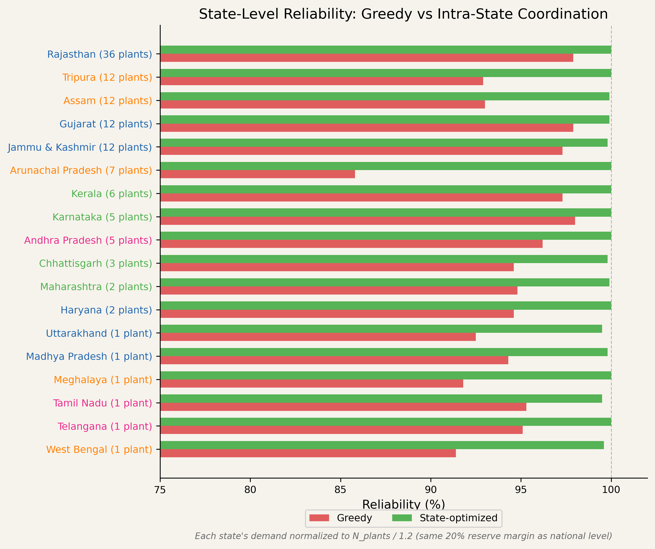
UC BERKELEY ANALYSIS · AUGUST 2026